---
title: "Measures of Central Tendency for an Asymmetric Distribution, and Confidence Intervals"
author:
- name: Frank Harrell
url: https://hbiostat.org
affiliation: Department of Biostatistics<br>Vanderbilt University School of Medicine
date: 2025-08-14
date-modified: last-modified
categories: [bootstrap, computing, inference, r, "2025"]
description: "There are three widely applicable measures of central tendency for general continuous distributions: the mean, median, and pseudomedian (the mode is useful for describing smooth theoretical distributions but not so useful when attempting to estimate the mode empirically). Each measure has its own advantages and disadvantages, and the usual confidence intervals for the mean may be very inaccurate when the distribution is very asymmetric. The central limit theorem may be of no help. In this article I discuss tradeoffs of the three location measures and describe why the pseudomedian is perhaps the overall winner due to its combination of robustness, efficiency, and having an accurate confidence interval. I study CI coverage of 18 procedures for the mean, one exact and one approximate procedure for the median, and five procedures for the pseudomedian, for samples of size $n=200$ drawn from a lognormal distribution. Various bootstrap procedures are included in the study. The goal of the confidence interval procedures is to achieve non-coverage probabilities that are close to the nominal 0.025 level in both tails. The usual standard deviation-based central limit theorem approach failed in both tails. The BCa bootstrap method was the most accurate for computing confidence limits for the mean, but the upper limit was too small with $n=200$, having non-coverage probability of 0.086 for the right tail instead of the nominal 0.025. No other bootstrap variants, including the fast triple studentized bootstrap, measureably improved confidence coverage. Three types of intervals for the more robust pseudomedian were extremely accurate, giving more reasons to use the pseudomedian as a primary location measure, whether or not the distribution is symmetric."
bibliography:
- grateful-refs.bib
code-fold: false
draft: false
---
# Measures of Central Tendency
For symmetric normal-like distributions there is a clear winner for measuring central tendency: the sample mean. The mean has the highest precision/efficiency and is also representative of a typical observation from the population distribution. The mean is not robust, e.g., is too affected by extreme values, when the distribution is heavy-tailed or asymmetric. [The sample mean has a breakdown point of 0, i.e., can be too affected by a single contaminated observation. The sample median has a breakdown point of 0.5, meaning it can withstand up to half of the observations being contaminated.]{.aside} For general continuous distributions with arbitrarily heavy tails or skewness, the sample median is robust and representative of a typical observation. But with a normal distribution the median is imprecise (higher variance, wider confidence limits) and has efficiency of only $\frac{2}{\pi} = 0.64$ compared to the mean. A sample of size 100 properly analyzed using a mean will revert to an effective sample size of 64 when using the median if normality holds.
For small samples the [Harrell-Davis smooth quantile estimator](https://academic.oup.com/biomet/article-abstract/69/3/635/221346) improves precision in estimating population quantiles. For the median, the HD estimate is the average sample median over infinitely many bootstrap resamples, although the algorithm is quite fast. It is implemented in the `Hmisc` package `hdquantile` function, which estimates the standard error of the estimate using the leave-out-one jackknife.
The [pseudomedian](https://en.wikipedia.org/wiki/Pseudomedian) (see also [here](https://en.wikipedia.org/wiki/Hodges–Lehmann_estimator)), also called the Hodges-Lehmann estimator, is less well known. It is affiliated with the Wilcoxon signed-rank test and can be computed by inverting that test, i.e., by finding the value that minimizes the signed rank statistic.[The pseudomedian has a breakdown point of 0.29]{.aside}. It is computed by taking all possible pairs of observations (including pairing an observation with itself), computing the midpoint of each pair, and computing the median of the midpoints. The R `Hmisc` package's `pMedian` function can compute the pseudomedian on 250,000 observations in 0.09 seconds.
When the distribution is normal, the efficiency of the pseudomedian compared to the mean is $\frac{3}{\pi} = 0.955$. When the distribution is symmetric, the pseudomedian is often much better than the sample mean or median in estimating the population mean and median. [Symmetry implies that the mean, median, and pseudomedian all estimate the same quantity, which is both the mean and the median since they are identical.]{.aside}
Let's see how often the pseudomedian is between the mean and median when sampling from a normal distribution of size $n=50$ and when the estimates non-trivially differ. Repeat for a lognormal distribution. Frequencies of `NA`s pertain to the number of samples (out of 5000) for which at least two of the three estimates were trivially different.
```{r}
require(Hmisc)
require(data.table)
require(boot)
require(bayesboot)
require(ggplot2)
options(datatable.print.class = FALSE)
g <- function(lognorm=FALSE) {
  x <- rnorm(50)
  if(lognorm) x <- exp(x)
  m    <- mean(x)
  med  <- median(x)
  pmed <- pMedian(x)
  mindif <- if(lognorm) 0.2 else 0.02
  dif <- min(diff(sort(c(m, med, pmed))))
  if(dif > mindif)
    (m < pmed & pmed < med) | (m > pmed & pmed > med)
  else NA
}
set.seed(1)
r <- replicate(5000, g())
table(r, useNA='ifany')
r <- replicate(5000, g(lognorm=TRUE))
table(r, useNA='ifany')
```
::: {.callout-note collapse="true"}
## Extension of the Pseudomedian to Difference Between Groups
When summarizing the difference between two independent groups of observations, we do not take the difference in pseudomedians, but instead use a more direct two-sample Hodges-Lehmann estimator: the median of all pairwise differences between an observation in group B and an observation in group A. This is the estimator that is zero when the Wilcoxon-Mann-Whitney two-sample test statistic is at its most null value.
It is always more difficult to estimate a difference than it is to estimate a one-sample quantity. Recall that in the normal case the variance of a difference in means equals the sum of the two variances. When there are $\frac{n}{2}$ observations in each of the two groups, the variance a mean of $n$ observations is $\frac{\sigma^{2}}{n}$ and the variance of the mean difference is $2 \times \frac{\sigma^{2}}{\frac{n}{2}} = \frac{4}{n}\sigma^{2}$. For the pseudomedian on $n$ observations we compute the median of $\frac{n (n + 1)}{2}$ midpoints. For differences in the balanced case we compute the median of $\frac{n ^{2}}{4}$ differences. The ratio of the number of one-sample pairs to the number of two-sample pairs is $\frac{2 (n + 1)}{n} \approxeq 2$ instead of the 4 in the parametric case. This takes into account that for the pseudomedian every pair shares an observation with other pairs.
:::
# Confidence Intervals
As discussed [here](https://stats.stackexchange.com/questions/186957), there is no nonparametric confidence interval for the mean of a general distribution. The mean is inherently a "parametric" quantity, unlike the sample median. Most data analysts mistakenly rely by default on the central limit theorem (CLT) to compute confidence limits for a population mean. A key problem arises: the population variance is seldom known. So analysts substitute the sample variance and proceed as if the variance is known, not aware they may be violating a key requirement of the CLT: the sample mean and sample variance must be independent in order for the standardized mean to converge with any rapidity to the normal distribution. For symmetric distributions this is OK, but not for asymmetric ones. Underlying this issue is that in practice one does not know how to transform the data to achieve normality, and we desire to estimate the population mean on the original scale. If the distribution were known to be lognormal, the analyst would analyze the data after taking logs. But there is no oracle to lead the analyst to this action, and if you should have taken logs but didn't, problems arise. Even if you knew to take logs, it is still a difficult problem to get confidence intervals for the population mean on the original scale (which is why the [smearing estimator](https://hbiostat.org/rmsc/areg#obtaining-estimates-on-the-original-scale) exists), although the formula for the population mean itself is a simple function of $\mu, \sigma$ on the log scale.
Proceeding without an oracle nearby, let $c$ be the 0.975 quantile of the normal distribution (1.96), and $s$ denote the sample standard deviation of the $n$ data values. Standard use of the CLT yields the following 0.95 confidence limits: $\bar{X} \pm c \times s / \sqrt{n}$. This formula is quite accurate even for $n$ as low as 20 when the data come from a normal distribution.
In all that follows we consider samples from the lognormal distribution with $\mu=0, \sigma=1.65$ on the log scale. As shown in [Biostatistics for Biomedical Research](https://hbiostat.org/bbr/htest#central-limit-theorem), the above CLT-based formula leads to very inaccurate confidence intervals. Even for $n=50,000$ the non-coverage in the two tails is 0.0182 on the left and 0.0406 on the right when both were supposed to be 0.025 for an overall 0.95 CI. Coverage is much worse for small $n$. Replacing $c$ with the critical value from a $t$ distribution will not help, as the problem is with asymmetry and not just heavy tails.
There are a number of ad hoc corrections to the CLT formula we will try. First, in recognition of asymmetry let's use dual SDs instead of a single sample SD. That is, compute $s_{1}$ by taking the observations that are below the sample mean and computing their root mean squared average distance from the overall mean $\bar{X}$ (we actually divide the sum of squares by one less than the number of low observations). Do likewise to compute $s_{2}$, the upper SD. Take the confidence limits to be $\bar{X} - c \times s_{1} / \sqrt{n}$ and $\bar{X} + c \times s_{2} / \sqrt{n}$, where $n$ is the overall sample size. Variations of this will also be tried, where instead of splitting on the mean we split on the median and on the pseudomedian.
Other ad hoc CI substitutes are tried below:
* Substitute Gini's mean difference for a single SD, scaling it by a factor that makes it estimate the SD unbiasedly if the distribution were normal
* Shift a confidence interval for the pseudomedian by the difference between the mean and pseudomedian
* Determine which quantiles of a standard normal distribution correspond to $c / \sqrt{n}$ and use those empirical quantiles from the raw data as the CI
* The same but use the Harrell-Davis quantile estimator
* Use 0.025 and 0.975 quantiles of the data shrunk towards the mean by a factor of $\sqrt{n}$.
But we expect that bootstrap confidence intervals will be more accurate, not to mention having better theory supporting them. [Charles Geyer has excellent presentations about the bootstrap and limitations of some of the bootstrap variants. See [this](http://users.stat.umn.edu/~geyer/boot.pdf) and [this](https://www.stat.umn.edu/geyer/3701/notes/bootstrap.html)]{.aside}. The problem is that there are many bootstrap variants. Based on theory and experience, the bias-corrected accelerated method called BCa is expected to perform best, because it explicitly handles asymmetry in sampling distributions. We can also add our own variations to the common bootstrap variants:
* When using normal approximation bootstraps based on bootstrap SDs of the estimates, substitute dual SDs as above
* Substitute the Harrell-Davis quantile estimator for nonparametric percentile bootstrap intervals
When using the sample median as the central tendency measure, there is for once an exact nonparametric confidence interval. The R function below computes it. This was taken from the [`DescTools` package](https://cran.r-project.org/web/packages/DescTools) `SignTest.default` function. See also [this](http://www.stat.umn.edu/geyer/old03/5102/notes/rank.pdf) and [this](http://de.scribd.com/doc/75941305/Confidence-Interval-for-Median-Based-on-Sign-Test).
```{r}
cimed <- function(x, alpha=0.05, na.rm=FALSE) {
  if(na.rm) x <- x[! is.na(x)]
  n <- length(x)
  k <- qbinom(p=alpha / 2, size=n, prob=0.5, lower.tail=TRUE)
  # Actual CL coverage: 1 - 2 * pbinom(k - 1, size=n, prob=0.5) >= 1 - alpha
  sort(x)[c(k, n - k + 1)]
  }
```
For the Harrell-Davis median estimator we assume normality and use the jackknife standard error to compute confidence limits.
Not studied here is _empirical likelihood_, which was a promising approach when it was developed by [Owen in 1990](https://en.wikipedia.org/wiki/Empirical_likelihood). But I tried it for the situation studied here and confidence coverage for the mean was terrible. Advocates of empirical likelihood suggested putting a bootstrap loop around the already computationally intensive combinatorial empirical likelihood algorithm, in order to get accurate CIs. But why go to that trouble instead of just using the bootstrap, or why not use the double bootstrap to get highly accurate intervals with much less computation than empirical likelihood?[The double bootstrap is used to correct a single bootstrap. The most efficient double bootstrap algorithm available increases computation time by $23\times$ over a single bootstrap.]{.aside}
**Update**: Various other boostrap variants were tried including a triple bootstrap, with unsatisfactory results. See a summary at the end of this article. This summary also better explains the fundamental limitations of mean-based methods for small skewed samples.
# Distribution and True Location Values
As mentioned above, the distribution from which we'll simulate samples is the lognormal distribution with $\mu=0, \sigma=1.65$.
```{r}
mu         <- 0
sigma      <- 1.65
truemean   <- exp(sigma ^ 2 / 2)
truemedian <- exp(mu)
```
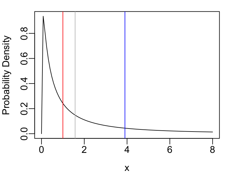
This is a highly skewed distribution with median $\exp(\mu) = 1.0$ and mean $\exp(\mu + \frac{1}{2}\sigma^{2}) =$ `r round(truemean, 4)`. There is no analytic expression available for the pseudomedian, so we compute it by simulating a sample of size $n=250,000$.
```{r}
set.seed(1)
truepmedian <- pMedian(rlnorm(250000, mu, sigma))
truepmedian
truevals <- c(mean = truemean, median = truemedian, pseudomedian = truepmedian)
```
The probability density function is shown below, with vertical lines depicting the three location measures (blue:mean, red:median, gray:pseudomedian).
```{r}
#| fig-width: 4
#| fig-height: 3
par(mar=c(3, 3, 1, 1), mgp=c(2, .43, 0))
curve(dlnorm(x, mu, sigma), 0, 8, ylab='Probability Density')
abline(v=truemean,    col='blue')
abline(v=truemedian,  col='red')
abline(v=truepmedian, col='gray')
```
# Distributions of Sample Location Estimates
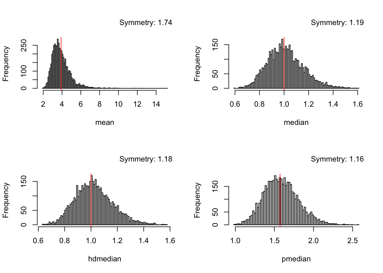
Let's see how much asymmetry exists in the distribution of sample estimates of central tendency by computing sample estimates from each of 5000 samples from our chosen log-normal distribution. Population values are shown with red vertical lines. Symmetry is quantified by the ratio of the SD of those values above the grand mean to the SD of those below.
```{r}
#| fig-width: 7
#| fig-height: 5
set.seed(1)
N <- 200
g <- function() {
  x <- rlnorm(N, mu, sigma)
  c(mean=mean(x), median=median(x), hdmedian=unname(hdquantile(x, 0.5)), pmedian=pMedian(x))
}
r <- t(replicate(5000, g()))
sym <- function(x) {
  s <- dualSD(x)
  ratio <- s['top'] / s['bottom']
  title(sub=paste('Symmetry:', round(ratio, 2)), line=-8, adj=1)
}

mmap <- .q(mean=mean, median=median, hdmedian=median, pmedian=pseudomedian)

par(mfrow=c(2,2))
for(p in colnames(r)) {
  u <- r[, p]
  hist(u, nclass=100, xlab=p, main=NULL); sym(u)
  abline(v=truevals[mmap[p]], col='red')
}
```
There is strong asymmetry in the sample means, which needs to be taken into account when constructing confidence limits which by necessity must also be asymmetric. Medians and pseudomedians have much more symmetric distributions.
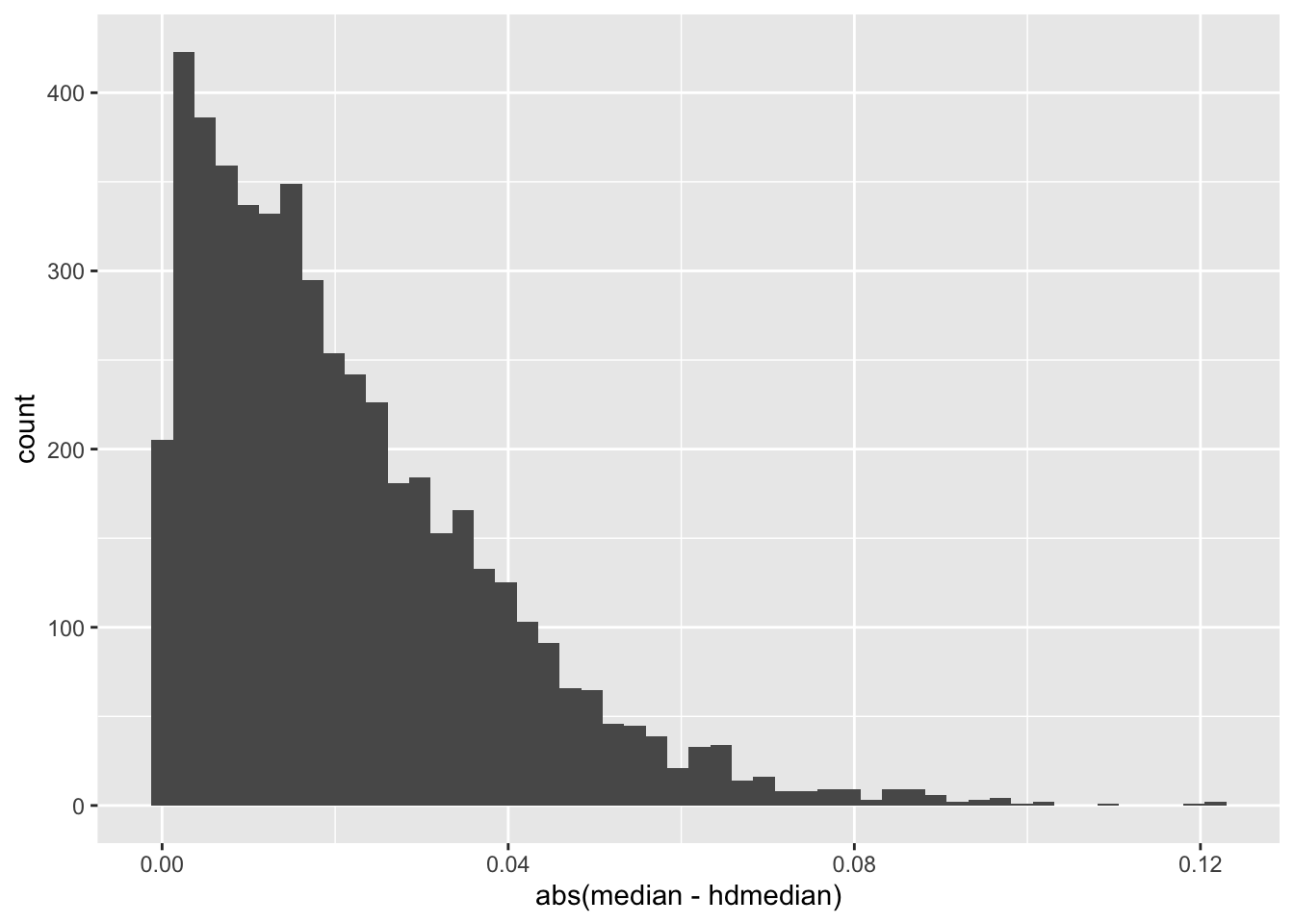
Out of curiosity, compare sample medians with Harrell-Davis estimates.
```{r}
ggplot(r, aes(x=abs(median - hdmedian))) + geom_histogram(bins=50)
```
Also compute the root mean squared error for the ordinary sample median vs. the HD median.
```{r}
rmse <- function(x) sqrt(mean((x - truemedian) ^ 2))
rmse(r[, 'median'  ])
rmse(r[, 'hdmedian'])
```
We see that for $n=`r N`$ the HD median was not worth the trouble. HD may have offered more precision for outer quantiles.
# CIs Computed for One Sample
Generate a sample of $n=`r N`$ from the chosen log-normal distribution and compute all the confidence limits we will study.
```{r}
w <- 'mean,CLT,usual
mean,CLT,dual SD pm
mean,CLT,dual SD med
mean,CLT,dual SD mean
mean,CLT,Gini
mean,boot,normal
mean,boot,basic
mean,boot,student
mean,boot,percentile
mean,boot,BCa
mean,boot,normal dual SD pm
mean,boot,normal dual SD med
mean,boot,normal dual SD mean
mean,boot,percentile HD
mean,boot,Bayesian
mean,shifted pm,
mean,CLT,percentile HD
mean,shrunk HD,
median,exact,
hdmedian,CLT,usual
pseudomedian,exact,
pseudomedian,boot,BCa
pseudomedian,boot,normal
pseudomedian,boot,percentile
pseudomedian,boot,basic'
what <- fread(text=w, col.names=c('measure', 'method', 'variant'), header=FALSE, fill=TRUE)
what[, type := 1 : nrow(what)]

cis <- function(x, exact=FALSE) {
  z     <- qnorm(0.975)
  m     <- mean(x)
  med   <- median(x)
  hdmed <- unname(hdquantile(x, 0.5, se=TRUE))
  pmed  <- pMedian(x)
  n     <- length(x)
  est   <- c(mean=m, median=med, hdmedian=hdmed, pseudomedian=pmed)
  estimate <- unname(what[, est[measure]])

  u <- z / sqrt(n)

  # nmin=10000 means use pooled SD if n < 100000
  dsd <- function(x, j) {
    dualSD(x, nmin=if(j == 1) 100000 else 2,
           center=switch(j, NA, pMedian(x), median(x), m ))
  }

  # Do all bootstrap resamples of the mean
  stat <- function(x, i) {
    x <- x[i]
    m <- mean(x)
    s <- sd(x)
    se <- s / sqrt(length(x))
    c(m, se)
  }
  b   <- boot(x, statistic=stat, R=1000)
  bmeans <- b$t[, 1]
  bci    <- boot.ci(b)[c('normal', 'basic', 'student', 'percent', 'bca')]
  lcl    <- function(z) z[length(z) - 1]
  ucl    <- function(z) z[length(z)]

  pmedb <- function(x, i) pMedian(x[i])
  # Do all bootstrap resamples of the pseudomedian
  bpm   <- boot(x, statistic=pmedb, R=1000)
  bpmci <- boot.ci(bpm, type=c('norm', 'perc', 'bca', 'basic'))

  # Create a list() of list()'s of computed lower and upper confidence limits so
  # that we can easily process all of them with sapply()
  res <- list(
    {
      # CLT
      lo <- hi <- numeric(4)
      for(j in 1:4) {
        s <- dsd(x, j)
        lo[j] <- m - u * s['bottom']
        hi[j] <- m + u * s['top']
      }
      list(lo=lo, hi=hi)
    },
    {
      # CLT using Gini's mean difference instead of SD
      s <- GiniMd(x) * sqrt(pi / 4)
      list(lo = m - u * s, hi = m + u * s)
    },
    list(lo = sapply(bci, lcl), hi = sapply(bci, ucl)),
    {
      # Bootstrap normal approximation CIs using dual SDs
      lo <- hi <- numeric(3)
      for(j in 2 : 4) {
        s <- dsd(bmeans, j)
        lo[j - 1] <- m - z * s['bottom']
        hi[j - 1] <- m + z * s['top']
      }
      list(lo=lo, hi=hi)
    },
    {
      # Bootstrap percentile CI using Harrell-Davis quantile estimator
      p <- hdquantile(bmeans, c(0.025, 0.975), names=FALSE)
      list(lo = p[1], hi=p[2])
    },
    {
      # Bayesian bootstrap
      wmean <- function(x, wts) sum(wts * x) / sum(wts)
      bb <- bayesboot(x, statistic=wmean, use.weights=TRUE, R=1000)
      s  <- summary(bb)
      list(lo=s$value[3], hi=s$value[4])
    },
    {
      # Compute shifted Hodges-Lehmann CI (shifted pseudomedian)
      w <- wilcox.test(x, conf.int=TRUE, exact=exact)
      shift <- m - w$estimate
      list(lo=w$conf.int[1] + shift, hi=w$conf.int[2] + shift)
    },
    {
      # CLT HD percentile
      p  <- pnorm(u)
      qu <- hdquantile(x, c(1 - p, 0.5, p))
      list(lo=m - qu[2] + qu[1], hi=m - qu[2] + qu[3])
    },
    {
      # Mean, shrunk Harrell-Davis 0.025 0..975 quantiles
      qu <- hdquantile(x, c(0.025, 0.975))
      w1 <- (m - qu[1]) / sqrt(n)
      w2 <- (qu[2] - m) / sqrt(n)
      list(lo = m - w1, hi=m + w2)
    },
    {
      # Exact nonparametric CI for median
      qu <- cimed(x)
      list(lo=qu[1], hi=qu[2])
    },
    {
      # HD approximate CI for HD median
      se <- attr(hdmed, 'se')
      list(lo=hdmed - z * se, hi=hdmed + z * se)
    },
    {
      # Exact nonparametric CI for pseudomedian under symmetry assumption
      w <- wilcox.test(x, conf.int=TRUE, exact=TRUE)
      list(lo=w$conf.int[1], hi=w$conf.int[2])
    },
    {
      # Bootstrap BCa confidence interval for the pseudomedian
      list(lo=lcl(bpmci$bca), hi=ucl(bpmci$bca))
    },
    {
      # Bootstrap normal approx for pseudomedian
      list(lo=lcl(bpmci$normal), hi=ucl(bpmci$normal))
    },
    {
      # Bootstrap percentile for pseudomedian
      list(lo=lcl(bpmci$percent), hi=ucl(bpmci$percent))
    },
    {
      # Basic bootstrap for pseudomedian
      list(lo=lcl(bpmci$basic), hi=ucl(bpmci$basic))
    }
    )

  lower <- unlist(sapply(res, function(x) x$lo))
  upper <- unlist(sapply(res, function(x) x$hi))

  data.table(type = 1:length(lower), estimate=estimate, Lower=lower, Upper=upper)
}

set.seed(2)
x <- rlnorm(N, mu, sigma)
cis(x)
```
# Simulation of CI Coverage
As an aside, many statisticians make the mistake of simulating only the overall confidence coverage to check against nominal levels such as 0.95. This can hide significant coverage errors in both tails, just because the two non-coverage probabilities may luckily sum to around 0.05. We will separately estimate non-coverage in each tail.
Run 5000 experiments using our chosen lognormal distribution.
```{r}
set.seed(3)
g <- function() {
  x <- rlnorm(N, mu, sigma)
  cis(x)
}
# Run reps simulations on one core
run1 <- function(reps, showprogress, core) {
  d <- data.table(sim = 1 : reps)
  r <- d[, g(), by=.(sim)]
  r[, sim := paste(core, sim, sep='-')]
  r
  }

if(file.exists('sim.rds')) R <- readRDS('sim.rds')  else {
  # The following tool 2 min. using 11 cores
  R <- runParallel(run1, reps=5000, seed=3)   # see https://hbiostat.org/rflow/parallel
  saveRDS(R, 'sim.rds')
}
```
Show distribution of confidence limits by method, separating means from other location measures. The spike histograms are interactive. Hover over elements to see more information.
```{r}
r <- copy(R)
r <- r[what, on=.(type)]
r[, z := paste(method, variant)]
curtail <- function(x, a, b) pmin(pmax(x, a), b)
s <- r[measure == 'mean',]
s[, Lower := curtail(Lower, -1, 9)]
s[, Upper := curtail(Upper, 2.5, 15)]
s[, histboxp(x=Lower, group=z, bins=200)]
s[, histboxp(x=Upper, group=z, bins=200)]
s <- r[measure != 'mean',]
s[, histboxp(x=Lower, group=paste(measure, z), bins=200)]
s[, histboxp(x=Upper, group=paste(measure, z), bins=200)]
# For a different look try:
# ggplot(R, aes(Lower, Upper)) + geom_bin2d(bins=150) +
#   viridis::scale_fill_viridis(trans='log10', option='inferno') + facet_wrap(~ type)
```
Check true values against means over simulations.
```{r}
mmap <- function(a) ifelse(a == 'hdmedian', 'median', a)
r[, trueval := truevals[mmap(measure)]]
r[, .(true = mean(trueval), mean_estimate = mean(estimate)), by=measure]
```
Compute non-coverage proportion for each tail for each method.
```{r}
error <- r[, .(low  = mean(Lower > trueval),
               high = mean(Upper < trueval)), by=.(measure, method, variant)]
```
Compute the total absolute error in the two tails.
```{r}
error[, total_error := abs(low - 0.025) + abs(high - 0.025)]
error
```
Compute the mean CI widths for the methods when estimating the mean. Print them in order of total coverage error.
```{r}
w <- r[measure == 'mean', .(length = mean(Upper - Lower)), by=.(measure, method, variant)]
u <- error[w, on=.(measure, method, variant)]
i <- u[, order(total_error)]
u[i, ]
# To display the table graphically use
# ggplot(u, aes(total_error, length, color=type)) + geom_point()
```
The overall winner for CI for the mean is the BCa bootstrap, which has tail non-coverage probabilities of 0.022 and 0.086 for overall coverage of 0.89 against the target of 0.95. This is not completely satisfactory, and a better confidence interval method may exist. If one wanted to trade off some coverage accuracy to get tighter CIs, the bootstrap percentile method might be considered. [As shown [here](https://stats.stackexchange.com/questions/186957), BCa yields poor coverage when $n=25$.
For $n=40$ and BCa again performed the best, but with 0.014 non-coverage on the left and 0.154 on the right. Even for $n=400$, no bootstrap variant got extremely close to 0.025 non-coverage in both tails, but BCa was still the best.]{.aside}
Ad hoc methods of computing confidence intervals for the mean had embarrassing performance. The usual CLT formula was unsatisfactory in both tails, and attempted fixes made things worse.
For the median, the exact nonparametric method works extremely well as advertised. The method based on the HD estimate and its standard error are satisfactory.
The real surprise comes from the performance of confidence intervals for the population pseudomedian. Both the classic exact Hodges-Lehmann confidence interval (which assumes symmetry of the population distribution) and the BCa bootstrap method were excellent, with BCa being almost perfect. The exact method probably works as well as it does because the sampling distribution of the pseudomedian for $N = `r N`$ was shown above to be very symmetric. The R `wilcox.test` will compute exact confidence limits for the pseudomedian quickly if $n < 1000$, and approximate confidence limits quickly if $n < 10,000$. Because BCa worked so well, and because the `pMedian` function is so fast for $n$ up to 250,000 (unlike the `wilcox.test` function), BCa would be a good default method. However BCa is slow for $n > 1000$, and a good replacement for it is the bootstrap nonparametric percentile CI in such cases. Beginning with `Hmisc` version 5.2-4, the `pMedian` function optionally efficiently computes bootstrap percentile (the default for $n \geq 150$) or BCa (the default for $n < 150$) confidence intervals.
::: {.callout-note collapse="true"}
## Timing and Agreement of Percentile and BCa Confidence Limits for Pseudomedian
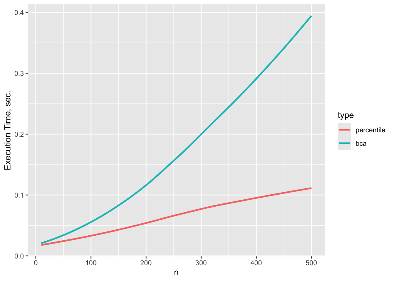
For varying sample sizes $n$ let's check agreement and execution time of two types of confidence limits for the pseudomedian. One thousand bootstrap resamples are used throughout.
```{r}
d   <- expand.grid(n=10:500, type=c('percentile', 'bca'))
setDT(d)
g <- function(n, type) {
  set.seed(n)   # make percentle and bca use the same data for each n
  y   <- rlnorm(n, mu, sigma)
  t1  <- system.time(a <- pMedian(y, conf.int=0.95, type=as.character(type)))['elapsed']
  list(time=t1, lower=a['lower'], upper=a['upper'])
}
if(file.exists('perc_vs_bca.rds')) u <- readRDS('perc_vs_bca.rds') else {
  u <- d[, g(n, type), by=.(n, type)]
  saveRDS(u, 'perc_vs_bca.rds')
}
ggplot(u, aes(x=n, y=time, color=type)) + geom_smooth(se=FALSE) +
  ylab('Execution Time, sec.')
```
Execution time is noticeably longer for BCa for $n > 200$.
```{r}
lo <- u[, lower]
hi <- u[, upper]
lim <- function(x) ylim(quantile(x, c(0.02, 0.98)))
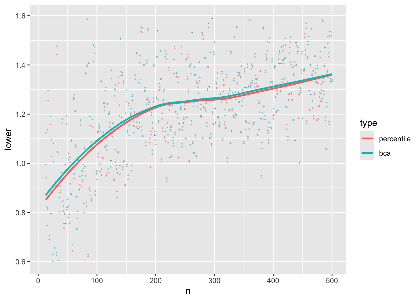
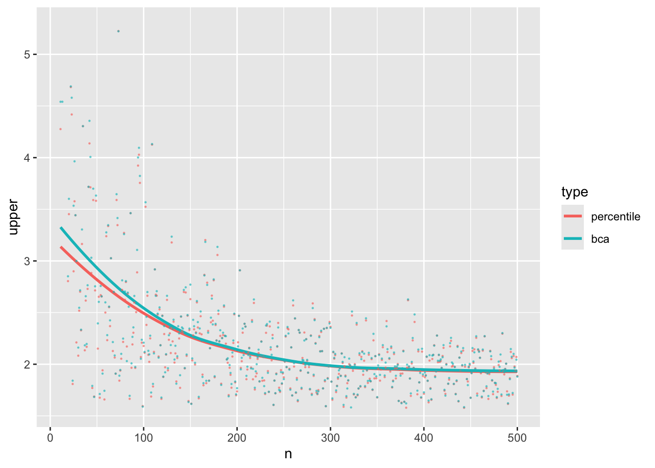
ggplot(u, aes(x=n, y=lower, color=type)) + geom_smooth(se=FALSE) +
geom_point(size=0.2, alpha=0.5) + lim(lo)
ggplot(u, aes(x=n, y=upper, color=type)) + geom_smooth(se=FALSE) +
  geom_point(size=0.2, alpha=0.5) + lim(hi)
```
Lower confidence limits for BCa and the percentile bootstrap are almost indistinguishable on average, especially for $n > 200$. Upper limits converge around $n=150$. This informs the default for the `Hmisc` `pMedian` function: BCa for $n < 150$ and percentile otherwise.
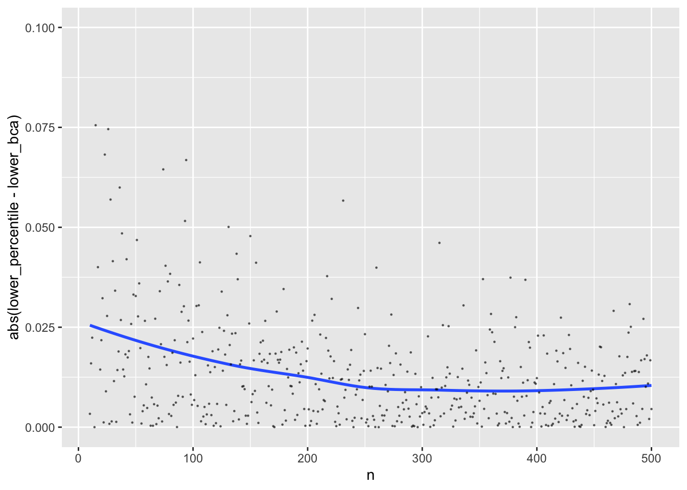
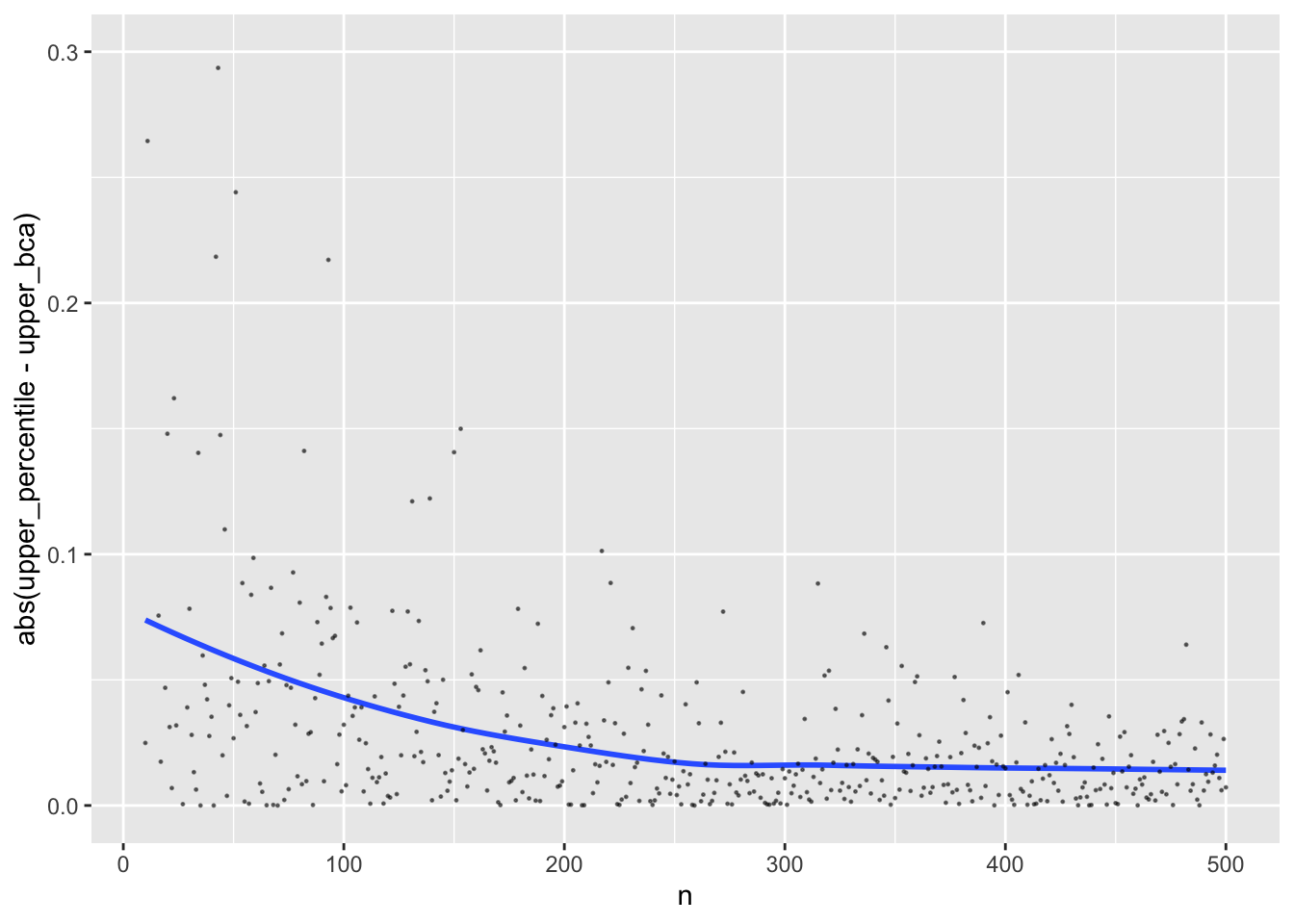
Instead of summarizing averages as was done above, look at individual sample differences between the two CI methods.
```{r}
w <- dcast(u, n ~ type, value.var=c('lower', 'upper'))
ggplot(w, aes(x=n, y=abs(lower_percentile - lower_bca))) + geom_smooth(se=FALSE) +
  geom_point(size=0.2, alpha=0.5) + ylim(0, 0.1)
ggplot(w, aes(x=n, y=abs(upper_percentile - upper_bca))) + geom_smooth(se=FALSE) +
  geom_point(size=0.2, alpha=0.5) + ylim(0, 0.3)
```
:::
::: {.callout-note collapse="true"}
## Width of "Exact" Confidence Intervals and Planning Studies for Precision
Compute the width of "exact" (under an assumption) CIs. Let the population pseudomedian be $\theta$ and assume that sample pseudomedians are from a location family such that they have a distribution that does not depend on $\theta$ (the population pseudomedian) but is then shifted by $\theta$. Let the zero-shift (underlying / standardized) sampling distribution be $g$. Then the exact 0.025 and 0.975 confidence limits of the pseudomedian are $[c - b, c - a]$ where $c$ is the sample pseudomedian, $a$ is the 0.025 quantile of $g$, and $b$ is the 0.975 quantile of $g$.[Note the similarity with the basic bootstrap.]{.aside} The width of the exact CI in this case is simply the difference in these outer quantiles, although the CI center moves with sample pseudomedians. Compute the quantiles and hence the width as a function of n by simulation.
```{r}
set.seed(1)
g <- function(n) pMedian(rlnorm(n, mu, sigma)) - truepmedian
tlim <- function(n) {
  pm <- t(replicate(3000, g(n)))
  qu <- quantile(pm, c(0.025, 0.975))
  list(q.025 = qu[1], q.975 = qu[2])
}
if(file.exists('real-lim.rds')) w <- readRDS('real-lim.rds') else {
  w <- data.table(n=10:500)
  w <- w[, tlim(n), by=.(n)]
  saveRDS(w, 'real-lim.rds')
}
w[, width := q.975 - q.025]
```
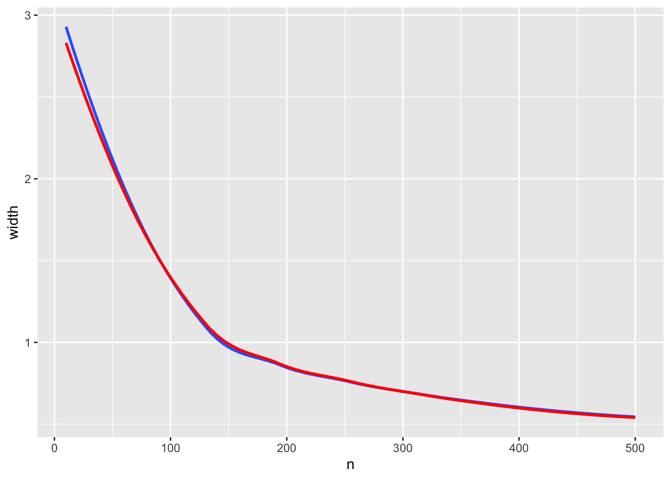
See if confidence limit widths following the $\sqrt{n}$ law.
```{r}
require(rms)
options(prType='html')
f <- ols(log(width) ~ log(n), data=w)
f
p <- exp(predict(f))
w[, pwidth := p]
ggplot(w, aes(x=n, y=width)) + geom_smooth(se=FALSE) +
  geom_smooth(mapping=aes(x=n, y=pwidth), se=FALSE, color=I('red'))
```
Exact widths are in blue, and true CI widths predicted by a log-log model are in red. There is excellent agreement. The fitted model to estimate the 0.95 CI width is approximately $14.32\times n^{-0.529}$, the last term being very close to $\sqrt{n} = n^{-0.5}$. This formula can be used for planning studies when the goal is to achieve a specified precision (half-width of the CI) in estimating the true pseudomedian when the population distribution is our lognormal distribution. For other distributions just replace the `g` function above with one specifying the distribution of interest, and use the simulated widths as a function of $n$ to solve for the minimum $n$ yielding adequate precision (margin of error).
:::
# Summary
The mean may be thought of as a "parametric quantity" and at present there is no general-purpose method for computing completely accurate (in both tails) confidence limits for means drawn from very asymmetric distributions. More methods for computing confidence limits for means are needed if you are likely to encounter very skewed distributions. The best available method at present is the BCa bootstrap, although its intervals are longer than some other methods.
The robustness and efficiency of the pseudomedian and the high accuracy of confidence limits for it (especially the bootstrap BCa and percentile limits) should make it more of a go-to measure of central tendency, for both symmetric and asymmetric distributions.
I hope that others will adapt the code provided here to study more sample sizes and distributions.
-----
# Confidence Intervals for the Mean Under Skewness: Why Every Fix We Tried Hit the Same Wall
The following was developed in an interaction with Claude Sonnet 4.6. The full chat with code and simulation results may be found [here](https://claude.ai/share/1c6e752f-d7ab-45f3-82a6-253d73a41d77).
## Starting point
We built `ftboot()`, an efficient R implementation of the fast triple bootstrap (FTB; Davidson & Trokić, 2020) for confidence intervals on the mean of a numeric vector. FTB approximates the (very expensive) standard triple bootstrap by replacing nested resampling with a single chain of three paired resamples per replicate, then inverting the resulting algorithm's nested order-statistic lookups in closed form rather than by numerical root-finding. The implementation was validated against a literal, unvectorized version of the published algorithm and showed good coverage and fast runtimes under ordinary (e.g., normal) data.
## The test that broke it
We then ran `ftboot()` on samples of size n=50 from a Lognormal(μ=0, σ=1) distribution, tracking left- and right-tail non-coverage separately (rather than just overall coverage, which can hide an imbalance between the tails). The result: the left tail was on target, but the right tail showed roughly double the nominal non-coverage rate. This matched what a plain BCa bootstrap also showed on the same data — and both findings echo Frank Harrell's much larger study (*Measures of Central Tendency for an Asymmetric Distribution, and Confidence Intervals*, fharrell.com/post/aci), which found that across 18 procedures for the mean (including CLT-based, several bootstrap variants, and ad hoc skewness corrections), BCa was the best performer yet still had right-tail non-coverage of 0.086 against a nominal 0.025 at n=200 for an even more skewed lognormal, with no method tested closing the gap even at n=400.
## What we tried, and why each attempt failed
**Skewness-adjusted bootstrap-t.** We tried layering a Johnson-style Edgeworth correction onto the studentized statistics feeding FTB's resampling chain, in two variants: adjusting only the bootstrap reference distribution, and adjusting both the reference distribution and the observed pivot. Neither helped; the first made the right tail meaningfully worse. The reason: Johnson's correction is designed to patch the gap between a t-statistic's true distribution and an idealized symmetric reference table — but the bootstrap-t already replaces that idealized reference with the empirical bootstrap distribution, which already encodes the data's skewness directly. Layering an analytic correction on top doesn't add information; it distorts an already-correct empirical picture, in this case by uniformly shifting the whole reference distribution in a way that narrowed the right tail rather than widening it.
**Switching the bootstrap variant (basic, percentile) instead of BCa.** Reasoned through rather than tested: both are expected to perform similarly or worse than BCa under skew, since BCa's whole design is to correct for exactly this asymmetry, and the simpler variants have no such correction at all.
**Transform, bootstrap, back-transform.** Bootstrapping log(x) and exponentiating the resulting interval endpoints gives a good CI for the *median* of X (or more precisely for exp of the log-scale mean), not for the *mean* of X — because the mean of a lognormal depends on both the log-scale mean and the log-scale variance, and naively exponentiating endpoints doesn't propagate the variance term's own uncertainty. This is a tool for a different estimand, not a shortcut to the same one.
**A flexible 3–4 parameter distributional family (e.g., GB2, generalized gamma, Tukey's g-h), fit by maximum likelihood, with the mean derived from the fitted parameters.** This relocates the problem rather than solving it: the mean's value under any of these families depends sensitively on the tail-shape parameter, and that parameter is estimated almost entirely from the few most extreme observations — the same scarce information that was starving the bootstrap's right tail in the first place. The family's flexibility helps only to the extent it is correctly specified, and verifying correct specification is hardest exactly where heavy tails make it matter most.
## The common thread
Every method above is, in a structural sense, doing the same thing: extrapolating into a region of the distribution that a finite, skewed sample under-represents. Nonparametric methods (bootstrap, empirical likelihood) are bound by the **support** of the n observed values — they cannot produce a tail more extreme than what was actually drawn. Parametric methods relocate that same limitation into the **precision of an estimated tail-shape parameter**, which is no better determined by a small sample than the support itself is. Frank Harrell independently found empirical likelihood gave "terrible" coverage for the same kind of problem, consistent with this diagnosis: it is the same ceiling, not a defect specific to bootstrapping or to EL.
The deeper reason is that **the mean is a linear functional of the data** — every observation, however extreme, contributes to it with full weight and no downweighting. A single far-out draw moves the mean by an amount proportional to its own size; nothing in the definition of the mean offers a cushion against that. Estimating it well under skew therefore *requires* getting the tail right, and getting the tail right from a finite sample is hard in direct proportion to how heavy and asymmetric that tail is. This is true whether the tail-fitting is done implicitly (resampling) or explicitly (a fitted shape parameter); the requirement doesn't go away, only the vocabulary used to describe it changes.
## The resolution: change the estimand, not the method
The median and the pseudomedian (Hodges-Lehmann estimator) are defined by **rank/order information** rather than by a weighted sum. The median doesn't care how extreme the largest observation is, only that it's larger than the others — so its sampling distribution stays close to symmetric and well-behaved even when the population is heavily skewed. This is a difference in *kind*, not degree: these estimators were never exposed to the tail-extrapolation problem that the mean cannot escape.
This matches Harrell's finding in the linked post: confidence intervals for the pseudomedian — both the BCa bootstrap version and the *exact* Hodges-Lehmann interval (which only assumes symmetry of the underlying distribution, not any particular parametric shape) — achieved near-nominal non-coverage in both tails at n=200 under the same lognormal distribution where 18 different procedures for the mean all fell short. The pseudomedian also retains most of the mean's efficiency under normality (95.5% relative efficiency) while having a breakdown point of 0.29, versus the mean's breakdown point of 0.
## Bottom line
For a continuous distribution of genuinely unknown and possibly asymmetric, heavy-tailed shape, no confidence interval procedure for the mean — bootstrap-based, analytically corrected, or built on a flexible parametric family — can be expected to reliably get both tails right at realistic sample sizes, because the difficulty is inherent to what the mean is, not to any particular method of estimating it. The pseudomedian (or median) sidesteps this problem entirely rather than mitigating it, which is the core argument for treating it as a primary measure of central tendency even when the data-generating distribution is not known to be symmetric.
## References
- Davidson, R. and Trokić, M. (2020). "The Fast Iterated Bootstrap." *Journal of Econometrics*, 218(2), 451–475.
- Harrell, F. (2025). "Measures of Central Tendency for an Asymmetric Distribution, and Confidence Intervals." *Statistical Thinking*. https://fharrell.com/post/aci
# Computing Environment
```{r}
grateful::cite_packages(pkgs='Session', output='paragraph', out.dir='.',
    cite.tidyverse=FALSE, omit=c('grateful', 'ggplot2'))
```
The code was run on `r sessionInfo()$running` on a Macbook Pro M2 Max.