A Comparison of Decision Curve Analysis with Traditional Decision Analysis
Introduction
In a traditional decision analysis, the analyst creates a decision tree and then estimates probabilities and assigns utilities for each possible outcome. Decision curve analysis is a type of decision analysis that can be applied to the evaluation of prognostic models and diagnostic tests. The major advantage is that it does not require specification of multiple utilities for different outcomes. Instead, the threshold probability of disease – a concept essential for clinical use of any model – is used to reflect the consequences of different decisions. The theory underlying decision curve analysis, and the use of threshold probability, has been discussed in multiple papers here, here, and here. The website decisioncurveanalysis.org includes links to these papers plus additional code, tutorials and data sets.
Here we compare decision curve analysis and traditional decision analysis to illustrate their similarities and differences.
Motivating example
We used the data set used in the evaluation of a commercial prostate cancer marker, the 4Kscore. We evaluated two prespecified models: the Prostate Cancer Prevention Trial (PCPT) risk calculator, described in the paper, and a new model (“Free PSA” model) consisting of total PSA, free PSA, prior negative biopsy, race and digital rectal exam. The aim of these models is to inform the decision to biopsy. A biopsy is seen as justified if it results in the detection of high-grade prostate cancer.
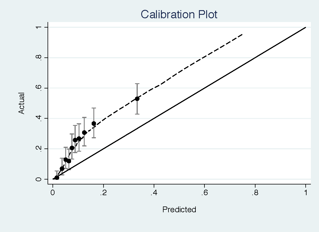
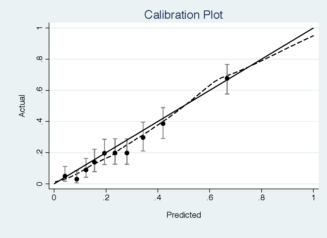
The PCPT model had a reasonable discrimination for high-grade prostate cancer (0.735) but was miscalibrated, with important underestimation of risk at low threshold probabilities (see top figure). The free PSA model has a slightly higher discrimination (0.774) but much better calibration, with only some slight overestimation of risk (bottom figure).
Traditional decision analysis
A traditional decision analysis starts with a tree, showing the decision point, given by a square, different outcomes, shown by a circle, and then outcomes. This is shown in the figure below. Here cancer is defined as “high-grade prostate cancer” and “no cancer” is benign findings or low-grade disease.
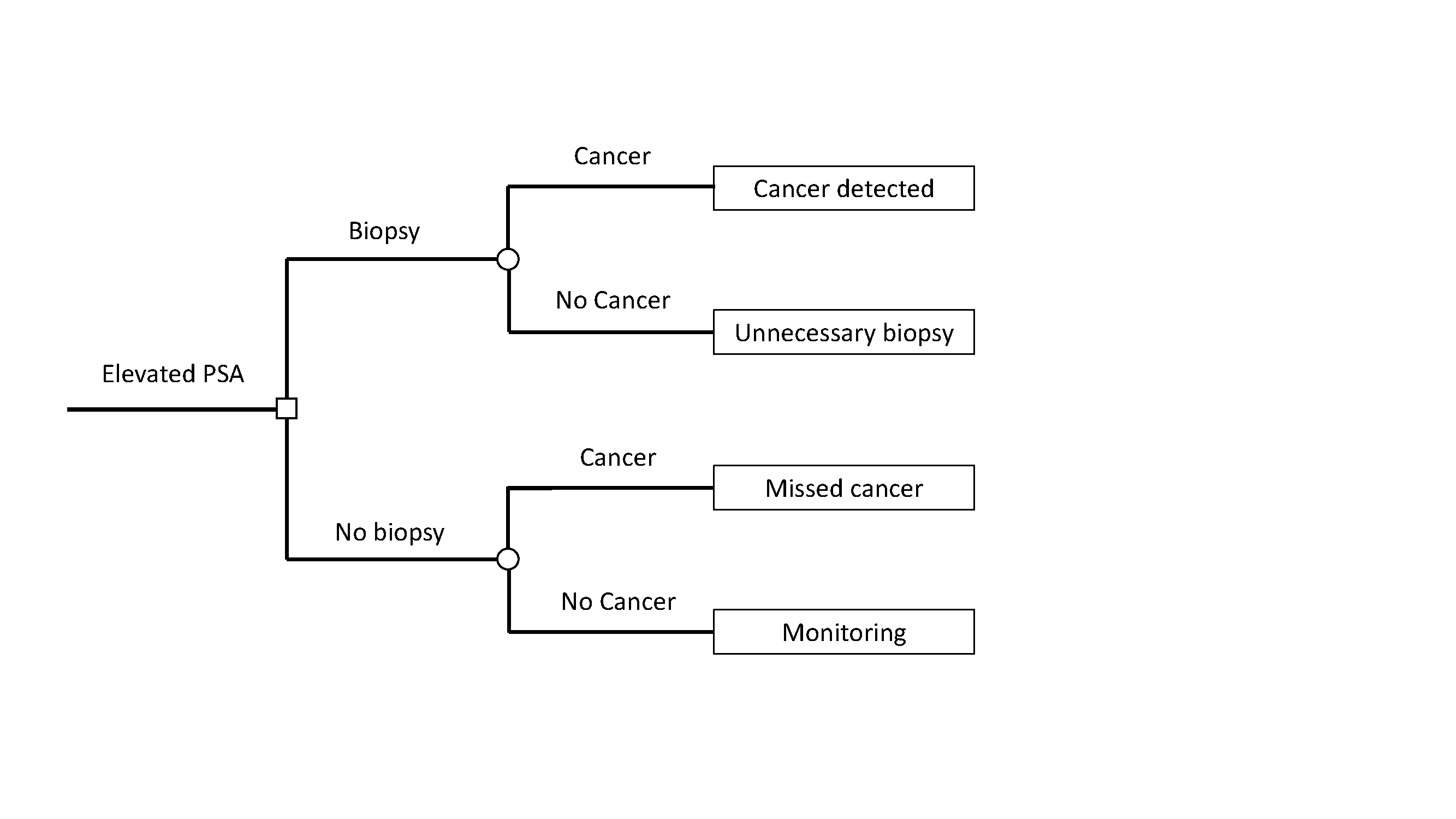
The next step is to assign utilities to each of the four possible outcomes. We can assign the outcome of no biopsy in a patient without cancer, the best possible outcome, the maximum utility of 1. A prostate biopsy is uncomfortable and is associated with a risk of infection, so an unnecessary biopsy is assigned a utility of 0.95. A diagnosis of high-grade cancer entails treatments such as radiotherapy and surgery, which can have long-term impacts on urinary, bowel and erectile function. A cancer diagnosis also raises the possibility of recurrent disease, with more toxic treatments such as hormonal therapy or chemotherapy, as well as the risk of metastasis and cancer-specific death. Hence finding a high-grade cancer will be assigned a utility of 0.8. Missing a cancer increases the risk of toxic treatment, metastasis and death and is assigned a utility of 0.35.
This is a somewhat simplified tree. A more complete tree might separate out low-grade from benign disease and then also allow for the possibility of biopsy complications, whether major or minor. This would lead to 12 different outcomes: high-grade / low-grade / no cancer detected on biopsy that leads to no / minor / major complications and no biopsy where the true disease state is high-grade / low-grade / no cancer. The simplified tree is used here as it better suited to help illustrate the underlying principles.
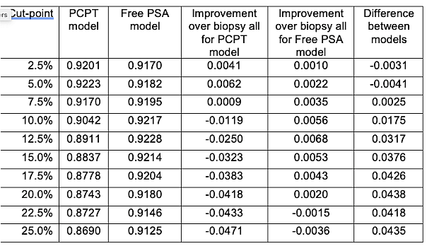
We can now apply the tree to the strategies of biopsying all men at risk – the current clinical strategy - biopsying no men, or biopsy according to the PCPT or free PSA prediction models. For the prediction models, we need to choose cut-points to determine what counts as a positive test indicating biopsy. The table shows utilities for different cut-points between a 2.5% and 25% risk of high-grade prostate cancer (there is actually a more rational way to choose the cut-point, but we will come back to that). The expected utility of biopsying all vs. no patients is 0.9161 and 0.8529 respectively. The table also shows the difference in expected utility between each model and the strategy of biopsying all men, and the difference in expected utility between the two models. The PCPT model is favored for low cut-points (2.5% and 5%) otherwise the highest expected utility is for the free PSA model.
Table 1
Decision curve analysis
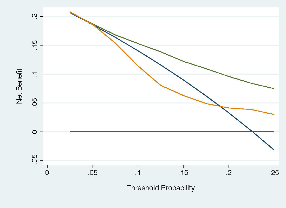
In a decision curve analysis, there is no need to consider and specify multiple different utilities, For the simplified tree, these would be the four utilities for true and false positives and negatives; for the more complete tree, described above, the analyst would have to specify, for instance, the utility of having a minor complication after biopsy in which low-grade cancer was found. Instead, all the analyst needs to do is obtain a range of reasonable probability thresholds. In the current case, that might be 5% - 20% (see this) although here we will show below a wider range for illustrative purposes. The free PSA model, shown in green, has much higher net benefit than the PCPT model (orange), which has lower net benefit than the strategy of biopsying all men (blue) for much of the range.
The net benefits are shown in table form below. Also shown is the net benefit calculated from the expected utilities in the first table using the formula (Expected utility of the model – utility of false negative) ÷ (utility of true positive – utility of false negative).
Table 2
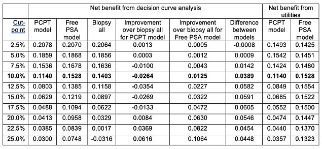
The critical point is that when the risk threshold is congruent with the utilities, net benefit calculated from a decision curve is the same as that calculated from utilities. This is shown in the bolded row. The rational risk threshold Pt can be obtained as Pt ÷ (1 - Pt ) = (utility of true positive – utility of false negative) ÷ (utility of true negative – utility of false positive). This gives Pt ÷ (1 - Pt ) = (utility of 0.8 – 0.35) ÷ (1 – 0.95) = 9 and hence Pt = 10%.
The table also shows that the rank ordering of utilities is altered when a cut-point is used that is inconsistent with the utilities. For instance, at a cut-point of 25%, the decision curve shows higher net benefit for the PCPT compared to the strategy of biopsying all men; the expected utility from the decision analysis favors biopsying all men. This can also be seen by comparing the strategies of treating all or no men. The decision curve analysis shows, appropriately, that the strategy of treating all men is only of higher net benefit if the threshold probability is below the prevalence.
Conclusion
We have compared traditional decision analysis with decision curve analysis. We show that, where the threshold probability in the decision curve analysis is congruent with the utilities used in the decision analysis, utility estimates are identical for both methods. We also show that decision curve analysis is a more natural fit for the evaluation of models because, unlike traditional decision analysis, there can be no inconsistency between the cut-point used for the model and the utilities used in the decision analysis.
Comments from Readers
Giuliano Cruz: Very interesting post! It hurts even more to read sens/spec “optimization” in, say, the biomarker literature after seeing decision theoretic approaches for specification of risk thresholds. One doubt I have: following https://www.tandfonline.com/doi/abs/10.1198/000313008X370302, the formula for rational odds(Pt) (that arrived at Pt=10%) seems inverted. As I read, it should be odds(Pt) = (TN-FP)/(TP-FN). Is that correct? Thanks!
Uriah Finkel: Great post! I wonder what about Risk Percentiles? In some applications it is required to observe results for top 5% population at risk, or that there’s enough budget for intervention for limited absolute amount of people. Should it be considered as another constraint?