---
title: "Parametric Models vs. Empirical Distributions and Ordinal Regression"
author:
- name: Frank Harrell
url: https://hbiostat.org
affiliation: Department of Biostatistics<br>Vanderbilt University School of Medicine
date: "2026-08-09"
date-modified: "last-modified"
categories: [data-science, inference, likelihood, ordinal, precision, regression, sample-size, "2026"]
description: "A primary goal of this article is to compare the accuracy of empirical cumulative distribution functions (ECDFs) and their logical extensions---cumulative probability ordinal regression models---with that of parametric distribution models when the population distribution may not be normal. A secondary goal is to derive an estimate of the effective degrees of freedom in play for ECDFs and ordinal model intercepts, by searching for the number of parameters in a parametric model that yields similar variance or mean squared error for probability estimates as the ECDF. Distribution-free methods minimize model specification risk and are broadly competitive with parametric models. It doesn't take much bias (lack of fit; underfitting) from a parametric model for it have worse mean squared error than a distribution-free method. Nonparametric and semiparametric estimation of a distribution function have major advantages and minor disadvantages over parametric models."
bibliography:
- grateful-refs.bib
code-fold: true
---
# Background
In modeling data we frequently need to estimate more than a mean. We may want to estimate quantiles, dispersion, or tail probabilities. These require model assumptions to be correct when the model is a smooth parametric one. Even when estimating a mean, for inference to be accurate we need distributional assumptions we make to be satisfied. The central limit theorem [offers no protection](https://fharrell.com/post/aci) especially when the underlying distribution is asymmetric.
Consider a continuous, discrete, or mixed-type random variable $Y$ having a cumulative distribution function $F(y) = P(Y \leq y)$. The empirical cumulative distribution function (ECDF) $F_{n}(y)$ defined below is the nonparametric maximum likelihood estimator of $F(y)$ from a sample of $Y$ values $Y_{1}, Y_{2}, \ldots, Y_{n}$.
$$F_{n}(y) = \frac{1}{n}\sum_{i=1}^{n} [Y_{i} \leq y]$$
where the indicator function $[u]$ is $1$ if $u$ is true, $0$ otherwise. The summation is just a count of the number of data values at or below $y$. The ECDF can be thought of as a cumulative histogram with no binning. It is uniquely defined and requires no choices to be made in its calculation.
There is a question of whether it is worth the trouble to fit a parametric distribution instead of relying on the ECDF. Does a parametric fit gain enough precision to offset the risk that the parametric distribution family may not adequately fit the data? Is it fair to think of the ECDF as essentially equivalent to a parametric estimator with several parameters capturing location, spread, skewness, heavy-tailedness, bimodality, and more? In other words does the variance of the ECDF mimic fitting a good many parameters to the distribution $F(y)$? How many parameters?
ECDFs and parametric distributions that don't have covariates are intended to be used for homogeneous samples and populations. To allow for heterogeneous tendencies in $Y$ we introduce covariates $X$. [Ordinal semiparametric regression models](https://hbiostat.org/ordinal) in the [cumulative probability model](https://fharrell.com/post/cpm) (CPM) family are covariate-shifted ECDFs so they inherit the distribution-free advantages of the ECDF. A CPM may be stated as
$$P(Y \leq y | X) = H(\alpha_{y} + X\beta)$$
where $H$ is some smooth increasing function, $\alpha$ is a vector of intercepts, $X$ is a vector of covariate values, $\beta$ are regression coefficients, and $|$ means "conditional on" or "given". Semiparametric models are distribution-free on the left side of the model and are parametric on the right side. [Ordinal CPMs could be called parametrically shifted (by $X\beta$) nonparametric models.]{.aside} Fortunately, the right side can be made arbitrarily flexible through the use of [spline functions and interaction terms](https://hbiostat.org/rmsc/genreg), with the only limitations coming from the effective sample size.
Common choices for $H$ are the logistic and normal cumulative distribution functions. There are as many intercepts as there are distinct $Y$ values, less one. This flexible vector of intercepts is what allows CPMs to fit any distributional shape. Whereas parametric models make _absolute_ distributional assumptions, semiparametric ones such as CPMs make only _relative_ distributional assumption, i.e., whatever shape $P(Y \leq y | X) = F(y | X)$ has, $H^{-1}(F(y | X))$ for different values of $X$ are assumed to be parallel. Parametric models assume that $H^{-1}(F(y | X))$ vs. $y$ is a straight line in addition to assuming the different straight lines for different $X$s are parallel.
When there are no covariates or $\beta=0$, the intercepts are just the $H$-inverses of the ECDF. So the ECDF is equivalent to a CPM with no covariates; $F_{n}(y) = H(\alpha_{y})$ for any $H$ when $\beta=0$. Accurate estimation of cumulative probabilities using CPMs goes hand-in-hand with accurate estimation of $F$ using an ECDF. One of our side aims is to estimate the effective number of parameters that the intercepts really involve.
The intercepts $\alpha_y$ are order-restricted, making them have far lower effective degrees of freedom than apparent at first. The order restriction also explains why one can fit a CPM with hundreds of thousands of intercepts extremely quickly, making CPMs work well for continuous $Y$ even for very large $n$. [The R `rms` package `orm` function can fit a model with $n=300,000$ and no ties in $Y$ (299,999 intercepts) and 10 covariates in 2.5 seconds.]{.aside}
Binary logistic regression is a special case of CPMs. It is virtually impossible to estimate $P(Y=1 | X)$ accurately unless you can estimate $\theta = P(Y=1)$ accurately. This requires an accurate estimate of the (single) intercept, which equates to estimating a simple probability $\theta$ with a proportion. When $\theta$ is unrestricted other than being forced to be in the interval $[0, 1]$, a confidence interval for $\theta$ has maximum width when $\theta=\frac{1}{2}$. So to have a good estimate of $\theta$ for all possible $\theta$ requires a good estimate when $\theta=\frac{1}{2}$. In this case, the sample size needed to estimate $\theta$ to within a margin of error of $\pm 0.1$ at the 0.95 confidence level is $n=96$. To have a margin of error of $\pm 0.05$ requires $n=384$.
# The Semi-Nonparametric (SNP) Density Family
Consider a continuous variable $Y$ with a continuous cumulative probability distribution $F$.
To compare the variance and mean squared error of the ECDF with a parametric family used to estimate $F(y)$, we need a family that incorporates a systematic progression from 2 parameters (mean and variance) to 3, 4, 5, ... . Such a family is the
[semi-nonparametric (SNP) density](https://www.jstor.org/stable/1913241) of Gallant & Nychka (1987).
This is a squared polynomial multiplying a standard normal kernel,
$$
f(x; \mu, \sigma, \theta) = \frac{\left[P_K(z)\right]^2 \phi(z)}{\sigma \, c(\theta)}, \qquad z = \frac{x - \mu}{\sigma}
$$
where $\phi$ is the standard normal density, $P_K(z) = 1 + \theta_1 z + \theta_2 z^2 + \cdots + \theta_K z^K$, and
$$
c(\theta) = \int_{-\infty}^{\infty} \left[P_K(z)\right]^2 \phi(z)\, dz
$$
is a normalizing constant. When $K = 0$ this reduces exactly to the ordinary Gaussian $N(\mu, \sigma^2)$, and each additional polynomial term adds one more shape degree of freedom — skewness, kurtosis, multimodality, and so on — while the squaring guarantees the density stays non-negative everywhere. As $K \to \infty$, this sequence is dense in a broad class of smooth densities, which is exactly why it's a natural tool for interpolating between "fully parametric" and "fully nonparametric" to study how many parameters it takes to approach ECDF-level behavior.
To fit an SNP distribution to data, the SNP parameters are estimated using maximum likelihood.
# Simulating Accuracy of $\hat{F}(\eta)$ for Population Median $\eta$
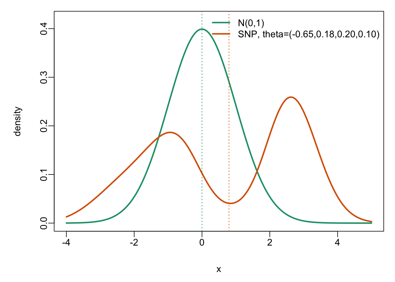
We simulate data from two very different continuous distributions, for varying sample sizes. The first distribution is the standard normal (Gaussian) $N(0, 1)$ distribution, which is the simplest SNP distribution ($K=0$). The second is an SNP distribution with $K=4$ for suitably chosen $\theta$ to result in a skewed bimodal distribution which will be plotted later. For each of 1000 samples for each $n$ and each data generating distribution we compute the ECDF and fit 7 SNP distributions, for $K=0,1,2,..., 6$. These SNP fits have $p=2,3,..., 8$ parameters.
From each estimator of $F(y)$ we estimate the accuracy of the estimated value $\hat{F}(y)$ at a single point for simplicity: the population median $\eta$. So we know that the true $F(y)$ at that point is $\frac{1}{2}$. We know that the ECDF is exactly unbiased for every distribution, so the expected value of ECDF$(\eta)$ = $\frac{1}{2}$. The variance of the ECDF at the true median is also known. It is $\frac{F(\eta)(1 - F(\eta))}{n} = \frac{1}{4n}$ which is also the mean squared error.
The following code was written by Claude Sonnet 5 after extensive interactions.
```{r}
##  1. p ranges 2..8, with new population-optimal starting
##     values computed for p=7,8 under both populations.
##  2. fit_snp_robust() is more robust: adds a larger-perturbation restart
##     (sd=0.8, not just 0.3) alongside the existing ones, since a targeted
##     check found ~24% of replicates had a meaningfully better optimum
##     than the previous 3-start search found.
##  3. Convergence is no longer just optim's internal flag. optim's
##     convergence=0 only means "my internal tolerance was satisfied" --
##     NOT that the fit is well-identified. A direct check found accepted
##     fits with Hessian condition numbers from the hundreds up to several
##     hundred thousand. fit_snp_robust() now also computes the condition
##     number of the winning fit's Hessian and returns it; sim() passes
##     this through as a companion "cond" vector rather than silently
##     dropping ill-conditioned fits to NA (that would risk a NEW,
##     undocumented selection bias -- e.g. if bad fits correlate with
##     particular samples). Downstream code can filter on `cond` explicitly
##     if desired, e.g. treating cond > 1e5 as unreliable.
##
## sim(n, psample) returns list(p, cdf, cond):
##   p    : 2:8
##   cdf  : F(m0; theta_hat) for each p (NA only on hard optimizer failure)
##   cond : condition number of the Hessian at the winning fit, for each p
##          (large values flag a weakly-identified fit -- inspect/filter
##          as needed; NOT pre-filtered here)

## =============================================================================
## SNP density family: g(z; theta) = P_K(z)^2 * phi(z) / c(theta)
## =============================================================================

poly_val <- function(z, theta) {
  K <- length(theta)
  out <- rep(1, length(z))
  if (K == 0) return(out)
  for (k in seq_len(K)) out <- out + theta[k] * z^k
  out
}

snp_norm_const <- function(theta) {
  if (length(theta) == 0) return(1)
  integrand <- function(z) poly_val(z, theta)^2 * dnorm(z)
  integrate(integrand, -Inf, Inf, rel.tol = 1e-9, subdivisions = 300)$value
}

snp_gcdf_scalar <- function(z0, theta, cst) {
  if (length(theta) == 0) return(pnorm(z0))
  integrate(function(u) poly_val(u, theta)^2 * dnorm(u), -Inf, z0,
            rel.tol = 1e-9, subdivisions = 300)$value / cst
}

snp_cdf <- function(x, mu, sigma, theta) {
  cst <- snp_norm_const(theta)
  z <- (x - mu) / sigma
  sapply(z, snp_gcdf_scalar, theta = theta, cst = cst)
}

unpack <- function(par) {
  list(mu = par[1], sigma = exp(par[2]),
       theta = if (length(par) > 2) par[3:length(par)] else numeric(0))
}

negloglik <- function(par, x) {
  pk <- unpack(par)
  cst <- snp_norm_const(pk$theta)
  if (!is.finite(cst) || cst <= 0) return(1e10)
  z <- (x - pk$mu) / pk$sigma
  dens <- poly_val(z, pk$theta)^2 * dnorm(z) / (cst * pk$sigma)
  if (any(!is.finite(dens)) || any(dens <= 0)) return(1e10)
  -sum(log(dens))
}

F_at <- function(par, x0, mu_fixed) {
  if (mu_fixed) return(pnorm(x0, mean = 0, sd = exp(par[1])))
  pk <- unpack(par)
  snp_cdf(x0, pk$mu, pk$sigma, pk$theta)
}

numgrad <- function(f, par, ...) {
  eps <- 1e-5 * pmax(abs(par), 1)
  g <- numeric(length(par))
  for (i in seq_along(par)) {
    pp <- par; pp[i] <- pp[i] + eps[i]
    pm <- par; pm[i] <- pm[i] - eps[i]
    g[i] <- (f(pp, ...) - f(pm, ...)) / (2 * eps[i])
  }
  g
}

delta_var <- function(fit, x0) {
  par  <- fit$par
  grad <- numgrad(F_at, par, x0 = x0, mu_fixed = fit$mu_fixed)
  cov  <- tryCatch(solve(fit$hessian), error = function(e) NULL)
  if (is.null(cov)) return(NA_real_)
  as.numeric(t(grad) %*% cov %*% grad)
}

## =============================================================================
## Populations
## =============================================================================

.build_population <- function(psample) {
  stopifnot(psample %in% c(2, 6))

  if (psample == 2) {
    TRUE_mu <- 0; TRUE_sigma <- 1; TRUE_theta <- numeric(0)
    m0 <- 0
    rdgp <- function(n) rnorm(n, TRUE_mu, TRUE_sigma)
    ## KL projection of N(0,1) onto any K>=0 polynomial family is theta=0.
    POP_START <- setNames(
      lapply(1:8, function(p) rep(0, if (p == 1) 1 else p)),
      as.character(1:8))
  }

  if (psample == 6) {
    TRUE_mu <- 0; TRUE_sigma <- 1; TRUE_theta <- c(-0.65, 0.18, 0.20, 0.10)
    true_cdf_tmp <- function(x) snp_cdf(x, TRUE_mu, TRUE_sigma, TRUE_theta)
    m0 <- uniroot(function(x) true_cdf_tmp(x) - 0.5, lower = -8, upper = 8, tol = 1e-12)$root
    stopifnot(abs(true_cdf_tmp(m0) - 0.5) < 1e-8)

    zgrid <- seq(-15, 15, length.out = 40001)
    dz    <- zgrid[2] - zgrid[1]
    dens_z_unnorm <- poly_val(zgrid, TRUE_theta)^2 * dnorm(zgrid)
    cdf_z_unnorm  <- cumsum(dens_z_unnorm) * dz
    cst_tab       <- cdf_z_unnorm[length(cdf_z_unnorm)]
    cdf_z         <- cdf_z_unnorm / cst_tab
    keep          <- !duplicated(cdf_z)
    qz            <- approxfun(cdf_z[keep], zgrid[keep], rule = 2)
    stopifnot(abs(cst_tab - snp_norm_const(TRUE_theta)) < 1e-3)
    stopifnot(abs(TRUE_mu + TRUE_sigma * qz(0.5) - m0) < 1e-3)
    rdgp <- function(n) TRUE_mu + TRUE_sigma * qz(runif(n))

    ## Population-optimal (KL-projection) starts, precomputed against this
    ## truth and hardcoded. p=6 is the exact truth. p=7,8 computed via
    ## direct numerical optimization (pop_fit_p78.R), p=1..5 as before.
    POP_START <- list(
      `1` = c(0.827706),
      `2` = c(0.649924, 0.785630),
      `3` = c(0.617291, 0.785658, 0.007438),
      `4` = c(0.604197, 0.126401, 0.031449, 1.068874),
      `5` = c(1.439483, 0.222466, 0.710348, 0.527649, -0.264142),
      `6` = c(TRUE_mu, log(TRUE_sigma), TRUE_theta),   # exact truth
      `7` = c(0.138567, 0.005169, -0.714358, 0.347910, 0.261525, 0.091971, -0.007512),
      `8` = c(0.792770, 0.055523, -0.140029, 1.435616, 0.218382, -0.069524, -0.030070, 0.006314)
    )
  }

  list(TRUE_mu = TRUE_mu, TRUE_sigma = TRUE_sigma, TRUE_theta = TRUE_theta,
       m0 = m0, rdgp = rdgp, POP_START = POP_START)
}

.POPULATIONS <- list(`2` = .build_population(2), `6` = .build_population(6))

## =============================================================================
## Robust MLE fit.
##   - starts: moment-based, population-optimal, and TWO random perturbation
##     scales (0.3 and 0.8) -- the larger scale was added because a direct
##     check found the smaller-only search missed a better optimum in about
##     a quarter of replicates.
##   - returns cond = condition number of the winning Hessian, so weakly-
##     identified "successes" are visible rather than silently accepted.
## =============================================================================

fit_snp_robust <- function(x, p_params, pop_start = NULL, n_random_starts = 2) {
  if (p_params == 1) {
    nll <- function(par) -sum(dnorm(x, mean = 0, sd = exp(par[1]), log = TRUE))
    starts <- list(log(sd(x)))
    if (!is.null(pop_start)) starts[[length(starts) + 1]] <- pop_start
    best <- NULL; best_val <- Inf
    for (st in starts) {
      op <- tryCatch(optim(st, nll, method = "BFGS", hessian = TRUE), error = function(e) NULL)
      if (!is.null(op) && op$convergence == 0 && op$value < best_val) { best <- op; best_val <- op$value }
    }
    if (is.null(best)) return(list(convergence = 1))
    return(list(par = best$par, hessian = best$hessian, p = 1,
                mu_fixed = TRUE, K = NA, convergence = best$convergence,
                cond = as.numeric(best$hessian) / as.numeric(best$hessian)))  # scalar -> cond=1
  }

  K <- p_params - 2
  starts <- list(c(mean(x), log(sd(x)), rep(0, K)))
  if (!is.null(pop_start)) starts[[length(starts) + 1]] <- pop_start
  scales <- rep(c(0.3, 0.8), length.out = n_random_starts)
  for (s in scales) starts[[length(starts) + 1]] <- c(mean(x), log(sd(x)), rnorm(K, 0, s))

  best <- NULL; best_val <- Inf
  for (st in starts) {
    op <- tryCatch(
      optim(st, negloglik, x = x, method = "BFGS",
            control = list(maxit = 3000, reltol = 1e-10), hessian = TRUE),
      error = function(e) NULL)
    if (!is.null(op) && op$convergence == 0 && op$value < best_val) {
      best <- op; best_val <- op$value
    }
  }
  if (is.null(best)) return(list(convergence = 1))
  eig <- tryCatch(eigen(best$hessian, only.values = TRUE)$values, error = function(e) NA)
  cond <- if (all(is.finite(eig)) && min(eig) > 0) max(eig) / min(eig) else Inf
  list(par = best$par, hessian = best$hessian, p = p_params, mu_fixed = FALSE,
       K = K, convergence = best$convergence, cond = cond)
}

## =============================================================================
## Reliability cutoff.
## optim's BFGS Hessian is itself typically only accurate to ~6 significant
## digits (finite-difference approximation), so trusting a condition number
## much beyond 1e6-1e7 is optimistic regardless of double-precision's
## theoretical ~1e15 budget. 1e6 is used as a round, defensible cutoff: it
## comfortably excludes the pathological cases (cond in the millions or Inf,
## seen at p=7,8) while keeping fits that are merely imprecise but still
## informative (e.g. psample=2, n=1000, p=6 averaged cond ~ 3e5 and matched
## the Monte Carlo result closely -- well under this cutoff).
## =============================================================================
COND_CUTOFF <- 1e6

## =============================================================================
## sim(n, psample): one Monte Carlo replicate, p = 2..8.
## cdf[p] is NA if the fit failed to converge
## =============================================================================

## =============================================================================
## sim(n, psample): one Monte Carlo replicate, p = 2..8.
## =============================================================================

sim <- function(n, psample = 2, i) {
  stopifnot(psample %in% c(2, 6))
  if(n == 25 && psample == 2)
    cat('n=', n, ' psample=', psample, ' i=', i, '\n', file='/tmp/z', append=TRUE)
  pop <- .POPULATIONS[[as.character(psample)]]
  x <- pop$rdgp(n)
  cdf <- cond <- dvar <- rep(NA_real_, 7)
  for (p in 2:8) {
    fit <- tryCatch(fit_snp_robust(x, p,
                                   pop_start = pop$POP_START[[as.character(p)]]),
                     error = function(e) list(convergence = 1))
    if (!is.null(fit$par) && fit$convergence == 0) {
      cond[p - 1] <- fit$cond
      cdf[p - 1]  <- F_at(fit$par, pop$m0, fit$mu_fixed)
      dvar[p - 1] <- tryCatch(delta_var(fit, pop$m0), error = function(e) NA_real_)
    }
  }
  list(p = 2:8, cdf = cdf, cond = cond, dvar = dvar)
}


## Example usage (uncomment to run):
## set.seed(1)
## sim(200, psample = 6)
##
## R <- 1000
## out <- t(replicate(R, { s <- sim(300, psample=6); c(s$cdf, s$cond) }))
## # first 7 cols = cdf estimates, next 7 = condition numbers -- inspect
## # cond before trusting cdf, e.g.: mean(out[,8:14] > 1e5, na.rm=TRUE)
```
Plot the probability density functions of these two data generating distributions. The normal distribution has $p=2$ fixed parameters: $\mu=0, \sigma=1$ and the skewed bi-modal SNP distribution has those parameters plus 4 fixed $\theta$ parameters for $p=6$ parameters in all. Also show the best fitting $K=2$ ($p=4$) distribution that approximates the $K=4$ one. This is the K-L projection of $K=4$.
```{r}
dens_fun <- function(x, mu, sigma, theta) {
  z <- (x - mu) / sigma
  if (length(theta) == 0) {
    dnorm(z) / sigma
  } else {
    cst <- snp_norm_const(theta)
    poly_val(z, theta)^2 * dnorm(z) / (cst * sigma)
  }
}

## K=2 (p=4) fit that most closely approximates (KL-projection of) the K=4
## (p=6) truth -- the population-optimal starting value already computed
## and hardcoded in POP_START[["4"]], re-verified above.
k2_par   <- c(mu = 0.604197, log_sigma = 0.126401,
              theta1 = 0.031449, theta2 = 1.068874)
k2_mu    <- k2_par["mu"]
k2_sigma <- exp(k2_par["log_sigma"])
k2_theta <- k2_par[c("theta1", "theta2")]
pop2 <- .POPULATIONS[["2"]]
pop6 <- .POPULATIONS[["6"]]

xg <- seq(-4, 5, length.out = 800)
d2 <- dens_fun(xg, pop2$TRUE_mu, pop2$TRUE_sigma, pop2$TRUE_theta)
d4 <- dens_fun(xg, k2_mu, k2_sigma, k2_theta)
d6 <- dens_fun(xg, pop6$TRUE_mu, pop6$TRUE_sigma, pop6$TRUE_theta)

par(mar = c(4.5, 4.8, 1, 1), mgp=c(2.8, .445, 0))
plot(xg, d2, type = "l", lwd = 2.5, col = "#1b9e77",
     ylim = c(0, max(d2, d4, d6) * 1.2),
     xlab = "x", ylab = "density",
     main = "")
lines(xg, d6, lwd = 2.5, col = "#d95f02")
lines(xg, d4, lwd = 2.5, col = "#7570b3", lty = 2)

abline(v = pop2$m0, col = "#1b9e77", lty = 3)
abline(v = pop6$m0, col = "#d95f02", lty = 3)

legend("topright",
       legend = c("psample=2: N(0,1)",
                  "psample=6: K=4 SNP, theta=(-0.65,0.18,0.20,0.10)",
                  "K=2 SNP approximating K=4"),
       col = c("#1b9e77", "#d95f02", "#7570b3"),
       lwd = 2.5, lty = c(1, 1, 2), bty = "n", cex = 0.85)
```
In the following code, `psample` denotes the value of $p$ (2 or 6) used to form a population distribution from which random draws are made.
Now run 1000 simulations for each combination of $n$ and `psample`.
```{r}
require(data.table)
require(Hmisc)
require(ggplot2)
ns <- c(25, 50, 75, 100, 150, 200, 250, 300, 400, 500, 750, 1000)

# Run reps simulations on one core
run1 <- function(reps, showprogress, core) {
  d <- expand.grid(n = ns, psample = c(2, 6),
                   i=paste(core, 1 : reps, sep='-'),
                   stringsAsFactors = FALSE)
  setDT(d)
  d[, sim(n, psample, i), by=.(n, psample, i)]
  }

# Don't let data.table use multi-threading which will clash with runParallel's
setDTthreads(1)

if(file.exists('sim.rds')) r <- readRDS('sim.rds') else {
  r <- runParallel(run1, reps=1000, seed=11)   # see https://hbiostat.org/rflow/parallel
  # Run time 4.1h using 11 cores
  saveRDS(r, 'sim.rds')
}
```
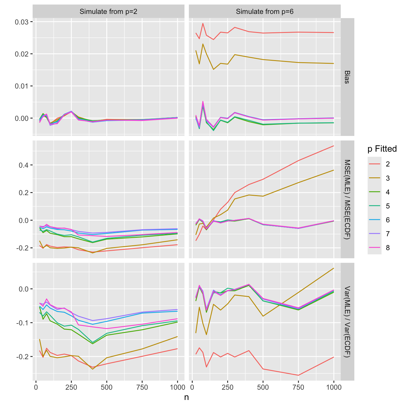
Plot the results after computing the following summary measures:
* Bias: mean estimate of F(population median) minus 0.5 (note the ECDF has zero bias)
* Relative Variance: $\log_{10}$ of the ratio of the simulated sample variances of the parametric estimator to the exact variance $\frac{1}{4n}$ of the ECDF, both computed at the population median
* Relative MSE: similar for the $\log_{10}$ of the ratio of MSEs
```{r}
g <- function(cdf, n) {
  cdf  <- cdf[! is.na(cdf)]
  bias <- mean(cdf) - 0.5
  v    <- log10(4 * n * var(cdf))
  mse  <- log10(4 * n * mean((cdf - 0.5) ^ 2))
  list(what = c('Bias', 'Var(MLE) / Var(ECDF)', 'MSE(MLE) / MSE(ECDF)'),
       est  =c(bias, v, mse))
}

w <- r[, g(cdf, n), by=.(n, psample, p)]
```
```{r}
#| fig-height: 7
#| fig-width: 7
#| column: screen-inset
ggplot(w, aes(x=n, y=est, color=factor(p))) + geom_line() +
  facet_grid(what ~ paste0('Simulate from p=', psample), scales='free_y') +
  guides(color=guide_legend(title='p Fitted')) + ylab('')
```
Consider the left three panels. All estimators of $\frac{1}{2}$ are unbiased because the $N(0,1)$ distribution is a special case of all SNP distributions, and because the ECDF is always unbiased. The bottom two panels show that for all sample sizes the parametric fits had better variance and mean squared errors (MSE) than the ECDF, since all log ratios of parametric:nonparametric ratios are negative. The performance of $p=6,7,8$ estimators is close to that of the ECDF, so one might roughly say that the ECDF has effectively 6 degrees of freedom in this situation.
Now consider the right three panels. With the data generating distribution being complex (including being bimodal), maximum likelihood estimates from parametric model fits with $p=2,3$ are very biased. The bias never wears off as $n\rightarrow \infty$ so the MSEs do not compete with the ECDF for $n>200$. Estimators with $p=4,5,6, 7, 8$ parameters all perform similarly with regard to MSE, and none has an advantage over ECDF. One could say roughly that the ECDF has effectively 4 parameters in this complex distribution setting.
## Integrated Mean Squared Error (IMSE)
Rather than comparing estimators at a single, arbitrarily chosen evaluation point, consider the integrated mean squared error (IMSE) of the estimate of a continuous $F(y)$ over the entire range of $y$. The IMSE approach measures fit quality across the *entire* distribution at once, weighted by where the population actually places its probability mass. For a parametric fitted CDF $\hat F_p$ with $p$ parameters, the integrated mean squared error is
$$
\text{IMSE}_p = E\left[\int \left(\hat F_p(x) - F(x)\right)^2\, dF(x)\right],
$$
where the weight $w(x)\,dx = dF(x)$ — i.e., averaging the squared error over $x$ drawn from the population itself, so regions with more probability mass contribute proportionally more to the comparison. This choice of weight is what gives the ECDF side of the comparison a clean closed form: since $\text{ECDF}(x)$ is unbiased for $F(x)$ with $\text{Var}[\text{ECDF}(x)] = F(x)(1-F(x))/n$,
$$
\text{IMSE}_{\text{ECDF}} = \int \text{Var}[\text{ECDF}(x)]\, dF(x) = \frac{1}{n}\int F(x)\big(1-F(x)\big)\, dF(x).
$$
Substituting $u = F(x)$ turns this into a distribution-free integral,
$$
\text{IMSE}_{\text{ECDF}} = \frac{1}{n}\int_0^1 u(1-u)\, du = \frac{1}{n}\left(\frac{1}{2}-\frac{1}{3}\right) = \frac{1}{6n},
$$
which holds *exactly*, for any continuous $F$, and so no simulation is required. $n \cdot \text{IMSE}_{\text{ECDF}}$ is exactly the classical Cramér–von Mises statistic, $\omega^2 = \int(\text{ECDF}(x)-F(x))^2\, dF(x)$, whose limiting mean is $\frac{1}{6}$. Because the ECDF benchmark is available in closed form, only the parametric side needs to be simulated: for each fitted model, $M$ fresh evaluation points are drawn from the population and $\text{IMSE}_p$ is estimated as $\frac{1}{M}\sum_j \left(\hat F_p(X_j) - F(X_j)\right)^2$.
```{r}
## =============================================================================
## CHANGED: .build_population -- adds cdf_fast, a fast forward CDF evaluator
## for the TRUE population (exact pnorm for psample=2; for psample=6, reuses
## the same tabulation already built for rdgp(), just read in the forward
## direction instead of inverted).
## =============================================================================

.build_population <- function(psample) {
  stopifnot(psample %in% c(2, 6))

  if (psample == 2) {
    TRUE_mu <- 0; TRUE_sigma <- 1; TRUE_theta <- numeric(0)
    m0 <- 0
    rdgp <- function(n) rnorm(n, TRUE_mu, TRUE_sigma)
    cdf_fast <- function(x) pnorm(x, TRUE_mu, TRUE_sigma)   # exact, no tabulation needed
    POP_START <- setNames(
      lapply(1:8, function(p) rep(0, if (p == 1) 1 else p)),
      as.character(1:8))
  }

  if (psample == 6) {
    TRUE_mu <- 0; TRUE_sigma <- 1; TRUE_theta <- c(-0.65, 0.18, 0.20, 0.10)
    true_cdf_tmp <- function(x) snp_cdf(x, TRUE_mu, TRUE_sigma, TRUE_theta)
    m0 <- uniroot(function(x) true_cdf_tmp(x) - 0.5, lower = -8, upper = 8, tol = 1e-12)$root
    stopifnot(abs(true_cdf_tmp(m0) - 0.5) < 1e-8)

    zgrid <- seq(-15, 15, length.out = 40001)
    dz    <- zgrid[2] - zgrid[1]
    dens_z_unnorm <- poly_val(zgrid, TRUE_theta)^2 * dnorm(zgrid)
    cdf_z_unnorm  <- cumsum(dens_z_unnorm) * dz
    cst_tab       <- cdf_z_unnorm[length(cdf_z_unnorm)]
    cdf_z         <- cdf_z_unnorm / cst_tab
    keep          <- !duplicated(cdf_z)
    qz            <- approxfun(cdf_z[keep], zgrid[keep], rule = 2)      # inverse: u -> z
    cdf_z_fwd     <- approxfun(zgrid, cdf_z, rule = 2)                  # forward: z -> u  (NEW)
    stopifnot(abs(cst_tab - snp_norm_const(TRUE_theta)) < 1e-3)
    stopifnot(abs(TRUE_mu + TRUE_sigma * qz(0.5) - m0) < 1e-3)
    rdgp <- function(n) TRUE_mu + TRUE_sigma * qz(runif(n))
    cdf_fast <- function(x) cdf_z_fwd((x - TRUE_mu) / TRUE_sigma)       # NEW (reuses same table)

    POP_START <- list(
      `1` = c(0.827706),
      `2` = c(0.649924, 0.785630),
      `3` = c(0.617291, 0.785658, 0.007438),
      `4` = c(0.604197, 0.126401, 0.031449, 1.068874),
      `5` = c(1.439483, 0.222466, 0.710348, 0.527649, -0.264142),
      `6` = c(TRUE_mu, log(TRUE_sigma), TRUE_theta),
      `7` = c(0.138567, 0.005169, -0.714358, 0.347910, 0.261525, 0.091971, -0.007512),
      `8` = c(0.792770, 0.055523, -0.140029, 1.435616, 0.218382, -0.069524, -0.030070, 0.006314)
    )
  }

  list(TRUE_mu = TRUE_mu, TRUE_sigma = TRUE_sigma, TRUE_theta = TRUE_theta,
       m0 = m0, rdgp = rdgp, cdf_fast = cdf_fast, POP_START = POP_START)   # cdf_fast added
}

.POPULATIONS <- list(`2` = .build_population(2), `6` = .build_population(6))

## =============================================================================
## NEW: fast_fitted_cdf -- fast tabulated CDF evaluator for a FITTED model,
## built once per fit (one grid pass), then answers any number of x-queries
## by interpolation instead of repeated integrate()-based F_at/snp_cdf calls.
## Falls through to exact pnorm for p=1,2, where no tabulation is needed.
## Did not exist before the IMSE change.
## =============================================================================

fast_fitted_cdf <- function(fit) {
  if (fit$mu_fixed) {
    sigma <- exp(fit$par[1])
    return(function(x) pnorm(x, 0, sigma))
  }
  pk <- unpack(fit$par)
  if (length(pk$theta) == 0) {
    return(function(x) pnorm(x, pk$mu, pk$sigma))
  }
  zgrid <- seq(-15, 15, length.out = 4001)
  dz    <- zgrid[2] - zgrid[1]
  dens_z_unnorm <- poly_val(zgrid, pk$theta)^2 * dnorm(zgrid)
  cdf_z_unnorm  <- cumsum(dens_z_unnorm) * dz
  cdf_z         <- cdf_z_unnorm / cdf_z_unnorm[length(cdf_z_unnorm)]
  keep          <- !duplicated(cdf_z)
  fwd           <- approxfun(zgrid[keep], cdf_z[keep], rule = 2)
  function(x) fwd((x - pk$mu) / pk$sigma)
}

## =============================================================================
## CHANGED: sim() -- adds the IMSE calculation. cdf/cond/dvar at m0 are still
## computed (now via the cheaper fast_fitted_cdf lookup instead of F_at for
## cdf specifically; cond and dvar still use the original fit_snp_robust /
## delta_var path, unchanged, since dvar genuinely needs F_at evaluated at
## perturbed PARAMETERS, which a fixed tabulation can't provide).
##   i : replicate index, used only for the debug log at n=25,psample=2
##   M : number of fresh evaluation points drawn per replicate (shared
##       across all p) to Monte-Carlo-approximate the integrated MSE
##       against dF(x). ECDF's own IMSE is closed-form: 1/(6n), no
##       simulation needed for that side of the comparison.
## =============================================================================

sim <- function(n, psample = 2, i, M = 300) {
  stopifnot(psample %in% c(2, 6))
  if(n == 25 && psample == 2)
    cat('n=', n, ' psample=', psample, ' i=', i, '\n', file='/tmp/z', append=TRUE)
  pop <- .POPULATIONS[[as.character(psample)]]
  x <- pop$rdgp(n)
  x_eval <- pop$rdgp(M)                  # NEW: fresh IID draw from the population, shared
  Ftrue_eval <- pop$cdf_fast(x_eval)     # NEW: across all p, for the IMSE comparison

  cdf <- cond <- dvar <- imse <- rep(NA_real_, 7)   # imse is NEW
  for (p in 2:8) {
    fit <- tryCatch(fit_snp_robust(x, p,
                                   pop_start = pop$POP_START[[as.character(p)]]),
                     error = function(e) list(convergence = 1))
    if (!is.null(fit$par) && fit$convergence == 0) {
      cond[p - 1] <- fit$cond
      dvar[p - 1] <- tryCatch(delta_var(fit, pop$m0), error = function(e) NA_real_)

      Fhat <- fast_fitted_cdf(fit)               # NEW: one tabulation per fit
      cdf[p - 1]  <- Fhat(pop$m0)                 # same quantity as before, cheaper to get
      imse[p - 1] <- mean((Fhat(x_eval) - Ftrue_eval)^2)   # NEW
    }
  }
  list(p = 2:8, cdf = cdf, cond = cond, dvar = dvar, imse = imse)
}
```
```{r}
setDTthreads(1)

if(file.exists('sim2.rds')) r <- readRDS('sim2.rds') else {
  r <- runParallel(run1, reps=1000, seed=13)
  # Run time 3.8h using 11 cores
  saveRDS(r, 'sim2.rds')
}
```
```{r}
g <- function(imse, n) {
  irmse <- sqrt(mean(imse, na.rm=TRUE))
  list(irmse = irmse,
       log.rel.irmse = log10(sqrt(6 * n) * irmse),
       diff = sqrt(1/(6*n)) - irmse)
}

w <- r[, g(imse, n), by=.(n, psample, p)]
# Add expected value of IMSE for ECDF
d <- expand.grid(n=ns, psample=c(2,6))
setDT(d)
d[, irmse := sqrt(1/6/n)]
d[, p := 0]
w <- rbind(w, d, fill=TRUE)
w[, p := ifelse(p == 0, 'ECDF', paste0('p=', p))]
w[, size := ifelse(p == 'ECDF', 1, 0.3)]

ggplot(w, aes(x=n, y=irmse, color=factor(p), size=I(size))) + geom_line() +
  facet_wrap(~ psample) +
  scale_y_log10(labels=scales::label_comma(),
                guide='axis_logticks') +
  guides(color=guide_legend(title='')) +
  ylab('Square Root IMSE')
```
<!--
ggplot(w, aes(x=n, y=log.rel.irmse, color=factor(p))) + geom_line() +
facet_wrap(~ psample) +
guides(color=guide_legend(title='p Fitted')) +
ylab('log10 Relative IRMSE')
ggplot(w, aes(x=n, y=diff, color=factor(p))) + geom_line() +
facet_wrap(~ psample) +
guides(color=guide_legend(title='p Fitted')) +
ylab('ECDF IRMSE - MLE IRMSE')
-->
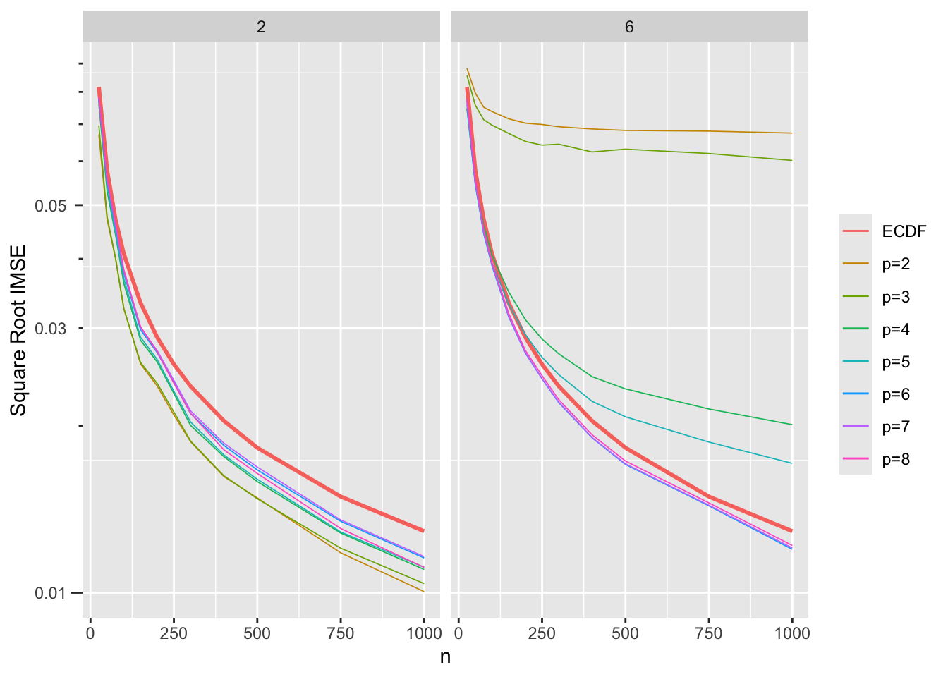
The square root of IMSE is shown. This is essentially a probability density-weighted average absolute error in estimating $F(y)$. Results for ECDF are shown with thicker lines and are identical across data generating distributions.
Consider first the left panel. When comparing the ECDF to easy-to-fit $N(0,1)$ data, there is separation at about $n=125$ when the ECDF is less accurate than all of the parametric estimators that have the normal distribution as a special case. ECDF performance is not very far from parametric $p=6,7,8$.
Now consider the right panel related to data simulated from a bimodal distribution with $p=6$. Maximum likelihood estimates of distribution parameters using $p=2,3$ seriously underfit the true $F(y)$ so are not competitive with the ECDF. Parametric estimates using $p=4, 5$ parameters did not perform as well as ECDF. The ECDF performed almost as well as $p=6, 7, 8$. One might say that the ECDF effectively has 6 parameters. For a CPM ordinal model one could likewise say that the large number of intercepts have effectively 6 degrees of freedom.
# Sample Size Requirements
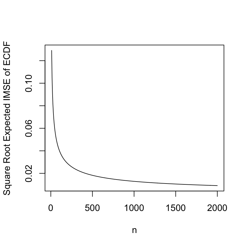
For estimating a mainly continuous $F(y)$ or for estimating the intercepts in a CPM, an average expected absolute error (actually the quadratic mean of $\sqrt{\text{IMSE}}$ across the whole distribution is $\sqrt{\frac{1}{6n}}$. A good target for a typical error in estimating $F(y)$ might be 0.025. This is achieved with $n=267$. To achieve a typical estimation error of 0.02 requires $n=417$. [In the ideal case of data coming exactly from a normal distribution, the sample size needed just to estimate $\sigma$ with a multiplicative margin of error of 1.1 at 0.95 confidence requires $n=233$ as detailed [here](https://hbiostat.org/bbr/htest#sec-htest-pilot-n).]{.aside}
```{r}
#| fig-height: 4.5
#| fig-width: 4.5
n     <- seq(10, 2000, by=5)
irmse <- sqrt(1/6/n)
plot(n, irmse, type='l', xlab='n', ylab='Square Root Expected IMSE of ECDF')
h <- function(n) round(sqrt(1/6/n), 4)
```
With $n=500$, $\sqrt{\text{IMSE}}$ of the ECDF is `r h(500)` and with $n=1000$ it is `r h(1000)`.
An adequate sample size means that one can estimate any cumulative probability fairly well, as well as quantiles. This applies to both ECDFs and CPMs. To ensure that covariate effect estimates also have sufficient accuracy, $n$ will have to be larger than the sample size needed for just the intercepts.
# Summary
Nonparametric (ECDF) and semiparametric (CPM) estimates are superior to parametric distribution estimators when the data generating distribution's complexities are not fully captured by the parametric model. When the data come from a simple distribution that is a special case of the parametric model, some precision is lost by the ECDF and by CPMs. But in general, distribution-free approaches are very competitive. We don't choose them because they are more precise under certain unknown conditions, but because their performance is exactly known and is independent of the shape of the data generating distribution. A parametric fit can do better as long as its bias is very small, but ECDFs and CPMs minimize model specification risk. Distribution-free estimators never perform poorly, and are not even relatively inefficient unless strong true assumptions are made for parametric estimators. When the distribution of $Y$ has floor or ceiling effects or discreteness, distribution-free estimation has even greater advantages.
# Resources
* [Empirical cumulative distribution function](https://en.wikipedia.org/wiki/Empirical_distribution_function)
* [General resources for ordinal models](https://hbiostat.org/ordinal)
* Gallant, A. R., & Nychka, D. W. (1987). [Semi-nonparametric maximum likelihood estimation](https://www.jstor.org/stable/1913241). *Econometrica*, 55(2), 363–390.
* [The unifying capabilities of cumulative probability semiparametric models](https://fharrell.com/post/cpm)
* [What does a statistical method assume?](https://fharrell.com/post/assume)
* [Measures of central tendency for an asymmetric distribution, and confidence intervals](https://fharrell.com/post/aci)
# Computing Environment
```{r}
grateful::cite_packages(pkgs='Session', output='paragraph', out.dir='.',
    cite.tidyverse=FALSE, omit=c('grateful', 'ggplot2'))
```
The code was run on `r sessionInfo()$running` on a Macbook Pro M2.