Seven Common Errors in Decision Curve Analysis
Introductory Remarks
In their classic paper on the evaluation of prediction models, Steyerberg et al. outlined a three-step process: discrimination, calibration, clinical utility. We first ask: does our model discriminate between those who do and don’t have disease? If so, we go on to ask: does the risk we give to an individual patient correspond to their true risk? But even if the answers to the first two questions are positive, we still have to ask whether using the model in clinical practice to aid clinical decision making would do more good than harm. Steyerberg at al. explicitly recommended decision curve analysis as a method to evaluate the clinical utility of models.
Decision curve analysis is now widely used in medical research. For instance, in 2022, PubMed finds over 1500 papers that used the phrase “decision curve analysis” in the abstract, and, of course, there will be many more papers using the method that do not use that exact phrase in the abstract. Naturally, decision curve analysis is sometimes used well, and sometimes less well. Below I discuss some of the more common errors in empirical practice. For more information on decision curve analysis, including code, tutorials, data sets and a bibliography of introductory papers, see www.decisioncurveanalysis.org.
Error 1: Failure to Specify the Clinical Decision
Statistical prediction models are most commonly created to inform either a specific medical decision or a small number of related decisions. For instance, a model to predict a patient’s risk of cancer is typically used to inform a decision to biopsy; a model to predict risk of postoperative complications might be used to select patients for “prehabilitation” (where risk is moderate) or to advise patients against surgery (where risk is high). Decision curve analysis evaluates those decisions, asking whether a patient’s clinical outcomes are improved if they follow the prediction model compared to the default strategies of “treat all” or “treat none”. However, if no decisions are specified by the investigators, then it becomes hard to see what the decision curve analysis is actually evaluating.
One exception is for general prognostic models intended for use in patient counselling. An example comes from cancer care. Cancer patients naturally ask “how long do you think I have, doctor?” because there all manner of personal decisions that will be based on the answer: Should I retire? Start that new project? Get my financial affairs in order? Go see my kids? Such models are the exception that proves the rule. Hence: A decision curve analysis should specify the decisions that would be informed by the model under study or, alternatively, state that it is a general prognostic model that would be used to inform a very wide range of personal decisions.
Error 2: Showing Too Wide a Range of Threshold Probabilities
It is not uncommon to see a decision curve analysis where the model is clearly intended to inform a specific decision, such as biopsy or prophylactic therapy, but the x axis includes a very wide range of threshold probabilities. Many of these threshold probabilities will be uninformative. For instance, there is no need to know the net benefit for a cancer prediction model at a threshold probability of 80%, because no reasonable decision-maker should demand an 80% risk of cancer before agreeing to biopsy. Unless they are evaluating a prognostic model used for general patient counseling, as described above, investigators should prespecify a limited range of reasonable threshold probabilities and limit the x axis to that range. A reasonable exception to this rule is if the lower bound of the threshold probability is low, such as 5% or 10%, in which case investigators may choose to start the x axis at 0.
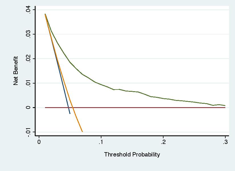
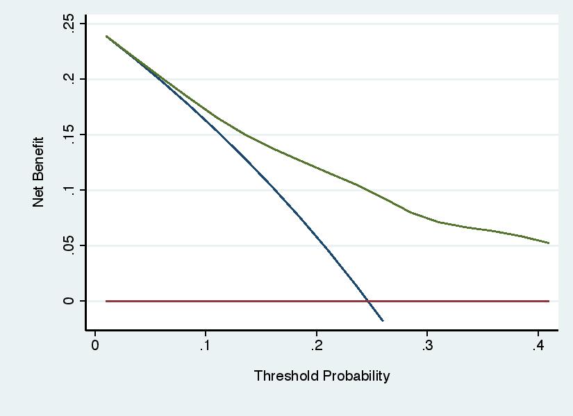
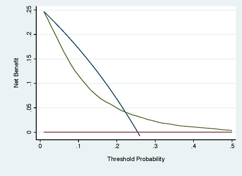
Error 3: Too Much White Space Below the \(x\)-axis
Negative net benefits are not very interesting. Investigators should truncate the y axis so that it starts at some negative level of net benefit, -0.01 is a typical choice, such that the graph shows where curves have negative net benefit without creating excessive white space below the y axis. the graph on the left (what you’d want to avoid) with that on the right (where the y axis is truncated, “ymin(-0.01)” in Stata, “ylim=c(-0.01,0.04)” in R).
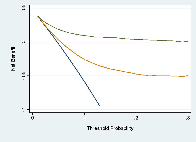
Unless you are careful, it is possible set the parameters of the graph so that a curve is left dangling above the x axis. For instance:
This is problematic because we need to know where net benefit becomes less than zero, albeit not how much less.
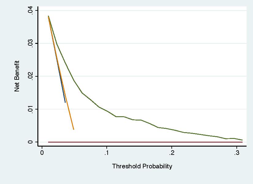
Error 4: Not Smoothing Out Statistical Noise
As threshold probability increases, net benefit should decrease smoothly until it reaches zero, at which point it may continue to decrease or, in some cases, remain zero for all higher values of threshold probability. When net benefit is calculated from a finite data set, however, statistical imprecision (“noise”) can cause local artifacts. It might be, for instance, that by chance, there are no patients who have a predicted probability at a given probability threshold, but then several have prediction probabilities at the next highest level and that causes a big difference in net benefit for a small change in threshold probability. This is shown on the left hand graph. In the right hand graph, net benefit has been set to be calculated every 2.5% (e.g. by “xby(0.025)” in Stata or “thresholds = seq(0, 0.4, 0.025)” in R) and a smoother has been added (e.g. “smooth” in Stata or “plot(smooth = TRUE)” in R). It should be noted that there is some disagreement between statisticians on this point. Some feel you should just “show the data”. My view is that the graph should reflect a best guess as to an underlying scientific truth and that would be a smooth curve without local artifacts.
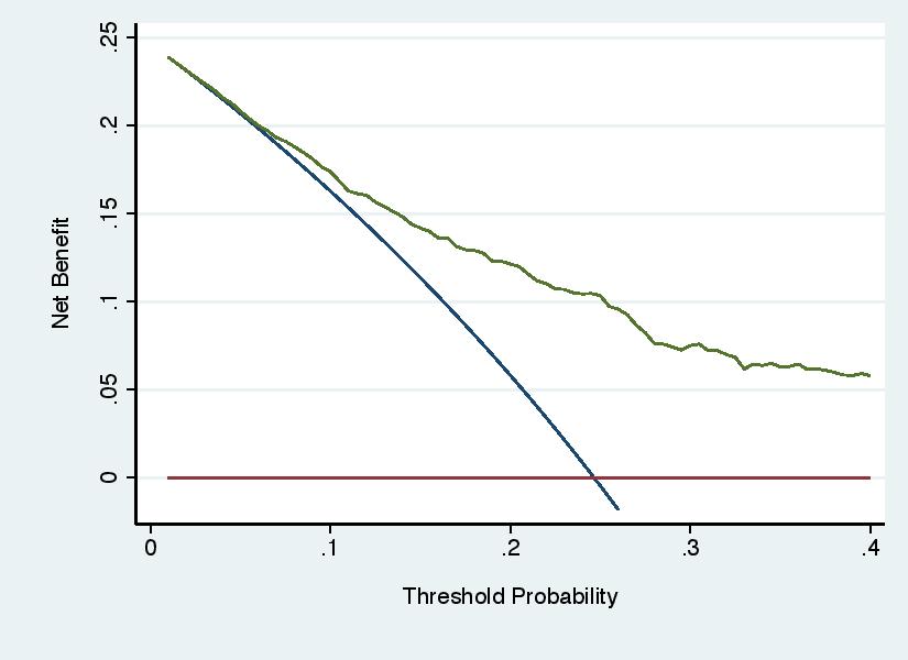
Error 5: Recommending Threshold Probabilities on the Basis of the Results
Decision curve analysis involves three steps: specifying a range of reasonable threshold probabilities; calculating net benefit across that range; determining whether net benefit is highest for the model across the complete range. Some investigators have used the results of the decision curve to choose the threshold probability for the model, rather than using the threshold probabilities to evaluate the model. For instance, see the graph below, a decision curve for a model to predict the outcome of cancer biopsy, where a wide range of threshold probabilities is shown for didactic purposes. Some authors might draw the incorrect conclusion that the model should be used with threshold probabilities of 25% - 50%. The correct conclusion would be that, as typical thresholds for biopsy would be around 10%, use of the model would do harm compared to the default strategy of biopsying all patients.
Error 6: Ignoring the Results
Decision curve analysis is not immune from the unfortunate tendency of investigators to ignore the actual results of a statistical analysis and declare success anyway. The decision curve shown under “Error 5” above clearly shows that the model should not be used to inform cancer biopsy, but an investigator might regardless state that the model “showed net benefit over a wide range of threshold probabilities”.
Error 7: Not Correcting for Overfit
Models created and tested on the same data set are prone to overfit, such that they appear to have better performance that they actually do. There are a number of simple and widely-used methods to correct for overfit. It is not uncommon that these are applied for calculation of discrimination (e.g. area-under-the-ROC-curve) but ignored for the decision curve. Authors can create predicted probabilities for each patient in a data set using a cross-validation approach and then use those probabilities for calculating both area-under-the-ROC-curve and net benefit for decision curve analysis. A methodology paper describing this approach has been published, with step-by-step instructions found in the tutorials at www.decisioncurveanalysis.org.