This article provides my reflections after the PCORI/PACE Evidence and the Individual Patient meeting on 2018-05-31. The discussion includes a high-level view of heterogeneity of treatment effect in optimizing treatment for individual patients.
Vanderbilt University School of Medicine Department of Biostatistics
Published
June 4, 2018
Modified
August 25, 2024
To translate the results of clinical trials into practice may require a lot of work involving modelling and further background information. ‘Additive at the point of analysis but relevant at the point of application’ should be the motto. — Stephen Senn When Relevance is Irrelevant
The simple idea of risk magnification has more potential to improve medical decision making and cut costs than “omics” precision medicine approaches. Risk magnification uses standard statistical tools and standard clinical variables. Maybe it’s not sexy enough or expensive enough to catch on.
Meeting critical care clinical trial guru Derek Angus for the first time1
Being with my long-time esteemed colleague Ewout Steyerberg
Hearing Cecile Janssens’ sanguine description of the information yield of genetics to date
Listening to Michael Pencina convey a big picture understanding of predictive modeling
Hearing Steve Goodman’s wisdom about risk applying to individuals but only being estimable from groups
Seeing Patrick Heagerty’s clear description of exactly what can be learned about an individual treatment effect when a patient can undergo only one treatment, and clearly discuss individual vs. population analysis
Hearing inspiring stories from two patient stakeholders who happen to also be researchers
Getting reminded of the pharmacogenomic side of the equation from my Vanderbilt colleague Josh Peterson
Watching John Spertus give a spirited report about how smart clinicians in one cardiovascular treatment setting are more likely to use a treatment for patients who stand to benefit the least, from the standpoint of predicted risk
Watching Rodney Hayward give an even more spirited talk about how medical performance incentives often do not achieve their intended effects
It was gratifying to hear extreme criticism of one-variable-at-a-time subgrouping from several speakers
It was worrying to see some speakers dividing predicted risk into quantile groups when in fact risk is a continuous variable, and quantile interval boundaries are driven by demographics (and are arbitrarily manipulated by changing study inclusion criteria) and not by biomedicine
1 One nit-picky comment about a small point in Derek’s presentation: He described an analysis in which a risk model was developed in placebo patients and applied to active arm patients. This approach has the possibility of creating a bias caused by fitting idiosyncrasies of placebo patients, in a way that may exaggerate treatment effect estimates.
Background Issues in Precision Medicine
There are five ways I can think of achieving personalized/precision medicine, besides the physician talking and listening to the patient:
Development of new diagnostic tests that contain validated, new information
Breakthroughs in treatments for well-defined patient sub-populations
Finding strong evidence of patient-specific treatment random effects using randomized crossover studies2, and finding actionable treatment plans once such heterogeneity of treatment effects (HTE) is demonstrated and understood
Finding strong evidence of interaction between treatment and patient characteristics, which I’ll call differential treatment effects (DTE)
Giving treatments to patients with the largest expected absolute benefit of the treatment (largest absolute risk reduction)
2 Stephen Senn has shown how one may estimate patient random effects representing individual response to therapy in a 6-period 2-treatment crossover study. See also this.
The last approach has little to do with HTE and is mainly a mathematical issue arising from the fact that there is only room to move a probability (risk) when the patient’s risk is in the middle. Patients who are at very low risk of a clinical outcome cannot have a large absolute risk reduction. I’ll call this phenomenon risk magnification (RM) because the absolute risk difference is magnified by having a higher baseline risk.
The conference focused more on RM than on HTE. RM is the simplest and most universal approach to medical decision making, and requires the least amount of information3. Before discussing RM vs HTE, we must define relative and absolute treatment effects. For a continuous variable such as blood pressure that is semi-linearly related to clinical outcome (at least with regard to the normal-to-hypertensive range of blood pressure), reduction in mean blood pressure as estimated in a randomized clinical trial (RCT) is both an absolute and a relative measure. For binary and time-to-event endpoints, an absolute difference is the difference in cumulative incidence of the event at 2y, or the difference in life expectancy. A relative effect may be an odds ratio, hazard ratio, or in an accelerated failure time model, a survival time ratio.
3 At least at the analysis phase, if not at the implementation stage.
Risk Magnification
There are two stages in the understanding and implementation of RM:
In an RCT, estimate the relative treatment effect and try to find evidence for constancy of this relative effect. If there is evidence for interaction on the relative scale, then the relative treatment effect is a function of patient characteristics.
When making patient decisions, one can easily (in most situations) convert the relative effect from the first step into an absolute risk reduction if one has an estimate of the current patient’s absolute risk. This estimate may come from the same trial that produced the relative efficacy estimate, if the RCT enrolled a sufficient variety of subjects. Or it can come from a purely observational study if that study contains a large number of subjects given usual care or some other appropriate reference set.
In most cases one can compute the absolute benefit as a function of (known or unknown) patient baseline risk using simple math, without requiring any data, once the relative efficacy is estimated. It is only at the decision point for the patient at hand that the risk estimate is needed.
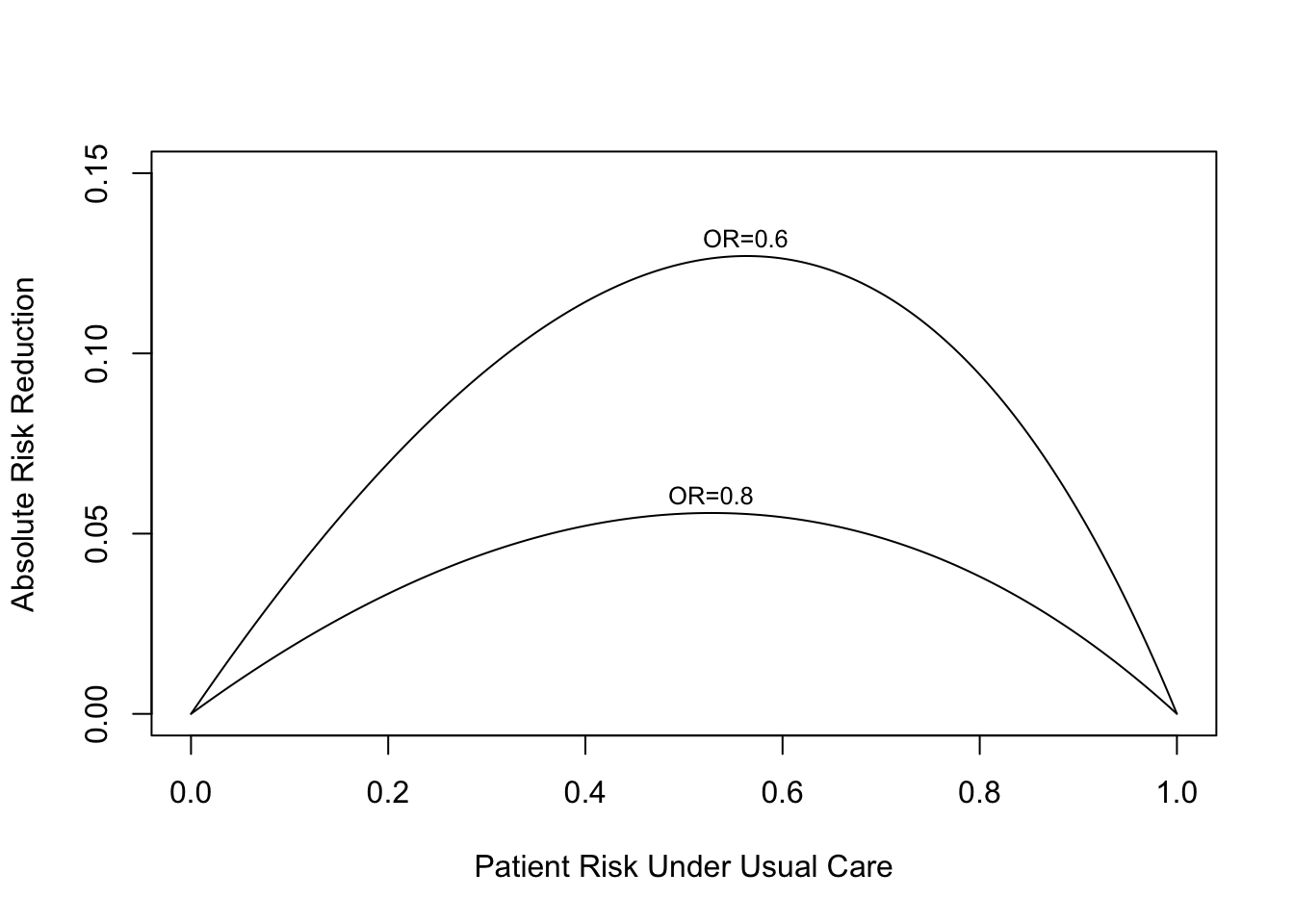
Here is an example for a binary endpoint in which the treatment effect is given by a constant odds ratio. The graph below exemplifies two possible odds ratios: 0.8 and 0.6. One can see that the absolute risk reduction by treatment is strongly a function of baseline risk (no matter how this risk arose), and this reduction can be estimated even without a risk model, under certain assumptions.
Code
require(Hmisc)plot(0, 0, type="n", xlab="Patient Risk Under Usual Care",ylab="Absolute Risk Reduction",xlim=c(0,1), ylim=c(0,.15))i <-0or <-c(0.8, 0.6)for(h in or) { i <- i +1 p <-seq(.0001, .9999, length=200) logit <-log(p/(1- p)) # same as qlogis(p) logit <- logit +log(h) # modify by odds ratio p2 <-1/(1+exp(-logit))# same as plogis(logit) d <- p - p2lines(p, d) maxd <-max(d) smax <- p[d==maxd]text(smax, maxd + .005, paste0('OR=', format(h)), cex=.8)}
For an example analysis where the relative treatment effect varies with patient characteristics, see BBR Section 13.6.2.
Heterogeneity of Treatment Effects
The conference did not emphasize the underpinnings of HTE, but this article gives me an excuse to describe my beliefs about HTE. In what follows I’m referring actually to DTE because I’m assuming that estimates are based on parallel-group studies, but I’ll slip into the HTE nomenclature.
It is only meaningful to define HTE on a relative treatment effect scale, because otherwise HTE is always present (because of RM) and the concept of HTE becomes meaningless. A relative scale such as log odds or log relative hazard is a scale in which it is mathematically possible for the treatment effect to be constant over the whole patient spectrum4. It is only the relative scale in which treatment effectiveness differences have the potential to be related to mechanisms of action. By contrast, absolute risk reduction comes from generalized risk, and generalized risk can come from any source including advanced age, greater extent of disease, and comorbidities. Researchers frequently make the mistake of examining variation in absolute risk reduction by subgrouping, one day shouting “older patients get more benefit” and another day concluding “patients with comorbidities get more benefit”, but these are illusory. It is often the case that anything giving the patient more risk will be related to enhancing absolute treatment benefit. It is an error in labeling to attribute these effects to a specific variable5.
4 Note that on an additive risk scale, interactions must be present to prevent risks from going outside the legal range of [0,1].
5 David Kent mentioned to me that he had some strong examples where relative treatment benefit was a function of absolute baseline risk. I need to know more about this.
Though the PCORI/Tufts meeting did not intend to cover the following topic, it would be useful at some point to have in-depth discussions about HTE/DTE, to address at least two general points:
Which sorts of treatment/disease combinations should be selected for examining HTE?
What happens when we quantify the outcome variation explained by HTE?
On the first point, I submit that the situations having the most promise for finding and validating HTE/DTE are trials in which the average treatment effect is large (and is in the right direction). It is tempting to try to find HTE in a trial with a small overall difference, but there are two problems in doing so. First, the statistical signal or information content of the data are unlikely to be sufficient to estimate differential effects6. Second, to say that HTE exists when the average treatment effect is close to zero implies that there must exist patient subgroups where the treatment does significant harm to the patients. The plausibility of this assumption should be questioned.
6 Under the best of situations, the sample size needed to estimate an interaction effect is four times that needed to estimate the average treatment effect.
On the second point, about quantification of non-constancy of relative treatment effect, a very fruitful area of research could involve developing strategies for “proof of concept” studies of DTE that parallels how principal component analysis has been used in gene microarray and GWAS research to show that a possible predictive signal exists in the genome. This same approach could be used to quantify the signal strength for differential treatment effects by patient characteristics. This would address a common problem: factors that potentially interact with treatment can be correlated, diminishing statistical power of individual interaction tests. By reducing a large number of potential interaction factors to several principal components (or other summary scores) and getting a “chunk test” for the joint interaction influence of those variables with treatment, one could show that something is there without spending statistical power “naming names.”
This relates to what I perceive is a major need in HTE research: to quantify the amount of patient outcome variation that is explained by treatment interactions in comparison to the variation explained by just using an additive model that includes treatment and a long list of covariates. A powerful index for quantifying such things is the “adequacy index” described in the maximum likelihood estimation chapter in Regression Modeling Strategies. This index answers the question “what proportion of the explainable outcome variation as measured by the model likelihood ratio chi-square statistic is explainable by ignoring all the intefraction effects?” One minus this is the fraction of predictive information provided by DTE. In my experience, the outcome variable explained by main effects swamps that explained by adding interaction effects to models. I predict that clinical researchers will be surprised how little differential treatment effects matter when compared to outcomes associated with patient risk factors, and when compared to RM.
My suggestions for developing statistical analysis plans for testing and estimating DTE/HTE are in BBR Section 13.6.
Averages vs. Customized Estimates
Advocates of precision medicine are required to show that customized treatment selection results in better patient outcomes than optimizing average outcomes.
An unspoken issue occurred to me during the meeting. We need to be talking much more about mean squared error (MSE) of estimates of individualized treatment effects. MSE equals the variance of an estimate plus the square of the estimate’s bias. Variance is reduced by increasing the sample size or by being able to explain more outcome variation (having a higher signal:noise ratio). Bias can come from a problematic study design that misestimated the average treatment effect, or by assuming that the effect for the patient at hand is the same as the average relative treatment effect when in fact the treatment effect interacted with one or more patient characteristics. But when one allows for interactions, the variance of estimates increases substantially (especially for patient types that are not well represented in the sample). So interaction effects must be fairly large for it to be worthwhile to include these effects in the model, i.e., for MSE to be reduced (i.e., for the square of bias to decrease more than the variance increases).
In the absence of knowledge about patient-specific treatment effects, the best estimate of the relative treatment effect for an individual patient is the average relative treatment effect7. Selecting the treatment that provides the best average relative effect will be the best decision for an individual unless DTEs are large. To better personalize the decision, other than accounting for absolute risk (which is a different issue and may objectively deal with cost issues), requires abundant data on DTE.
7 This can be easily translated into a customized absolute risk reduction estimate as discussed earlier.
Generalizability of RCTs
At the meeting I heard a couple of comments implying that randomized trials are not generalizable to patient populations that are different from the clinical trial patients. This thought comes largely from a misunderstanding of what RCTs are intended to do, as described in detail here: to estimate relative efficacy. Even though absolute efficacy varies greatly from patient to patient due to RM, evidence for variation in relative efficacy has been minimal outside of the molecular tumor signature world.
The beauty of the conference concentrating on risk magnification is that RM always exists whenever risk is an issue (not so much in a pure blood pressure trial), RM is easier to deal with, and to account for RM does not require increasing the sample size, although RM is benefited from having large observational cohorts upon which to estimate risk models for computing absolute risk reduction given patient characteristics and relative treatment effects. RM does not require crossover studies, and can be actualized even without a risk model if the treating physician has a good gestalt of her patient’s outcome risk. In my view, RM should be emphasized more than HTE because of its practicality. To do RM “right” to obtain personalized estimates of absolute treatment benefit, we do need to spend more effort checking that risk models are absolutely calibrated.
Other Things I’d Like to Have Heard or Further Discussed
There was some discussion of multiple endpoints and tradeoffs between safety and efficacy. Patient utility analysis and the use of ordinal clinical outcomes would have been a nice addition, though there’s not time for everything.
The ACCORD-BP trial was described as “negative”, but that was a frequentist trial so all one can say is that the trial did not amass enough information to reject the null hypothesis.
I heard someone mention at one point that subgroup analysis “breaks the randomization.” I don’t think that’s strictly true. It’s just that subgroup analysis is not competitive statistically, and is usually misleading because of noise, arbitrariness, and co-linearities.
Someone mentioned tree methods but single trees require 100,000 patients to work adequately and even then are not competitive with regression.
There needs to be more discussion about the choice of outcome measures in trials. DTE/HTE analysis requires high-information outcomes to have much hope; binary outcomes have low information content.
It may have been Fan Li and Michael Pencina who mentioned the use of penalized maximum likelihood estimation for estimating DTE (e.g., lasso, elastic net). These do not provided any statistical inference capabilities (as opposed to Bayesian penalization through skeptical priors).
Evidence for Homogeneity of Treatment Effects
For continuous outcome variables Y where the variance of measurements can be disconnected from the mean, one way to estimate the magnitude of HTE is to compare the variance in Y in the active treatment group and that in the control group. If HTE exists, it cannot affect a pure control group but should increase the variance of Y in the treatment group due to heterogeneity of treatment effect across types of subjects. Two studies have examined this issue in meta-analyses. The first, related to weight loss treatments, found “evidence is limited for the notion that there are clinically important differences in exercise-mediated weight change.” The second paper reviewed 208 studies and found evidence in the opposite direction from HTE: the average ratio of variances of Y for treated:control was 0.89.
---title: Viewpoints on Heterogeneity of Treatment Effect and Precision Medicineauthor: - name: Frank Harrell url: https://hbiostat.org affiliation: Vanderbilt University<br>School of Medicine<br>Department of Biostatisticsdate: 2018-06-04date-modified: 2024-08-25categories: [RCT, biomarker, decision-making, drug-evaluation, generalizability, medicine, metrics, personalized-medicine, prediction, subgroup, 2018]description: "This article provides my reflections after the PCORI/PACE Evidence and the Individual Patient meeting on 2018-05-31. The discussion includes a high-level view of heterogeneity of treatment effect in optimizing treatment for individual patients."---::: {.quoteit}To translate the results of clinical trials into practice may require a lot of work involving modelling and further background information. 'Additive at the point of analysis but relevant at the point of application' should be the motto.<br>— Stephen Senn [When Relevance is Irrelevant](http://errorstatistics.com/2013/04/19/stephen-senn-when-relevance-is-irrelevant)<br><br>The simple idea of risk magnification has more potential to improve medical decision making and cut costs than "omics" precision medicine approaches. Risk magnification uses standard statistical tools and standard clinical variables. Maybe it's not sexy enough or expensive enough to catch on.:::## Notes on the PCORI/Tuft PACE MeetingThis is a reflection on what I heard and didn't hear at the 2018-05-31 meeting [Evidence and the Individual Patient: Understanding Heterogeneous Treatment Effects (HTE) for patient-Centered Care](https://nam.edu/event/evidence-and-the-individual-patient-understanding-heterogeneous-treatment-effects-for-patient-centered-care), sponsored by [PCORI](https://pcori.org), the Tufts University [PACE Center](https://www.tuftsmedicalcenter.org/Research-Clinical-Trials/Institutes-Centers-Labs/Institute-for-Clinical-Research-and-Health-Policy-Studies/Research-Programs/Center-for-Predictive-Analytics-and-Comparative-Effectivness.aspx), and the [National Academy of Medicine](http://nam.edu). I learned a lot and thought that the meeting was well organized and very intellectually stimulating. Hats off to David Kent for being the meeting's mastermind. Some of the high points of the meeting to me personally were [[Comments](https://hbiostat.org/comment.html)]{.aside}* Meeting critical care clinical trial guru Derek Angus for the first time^[One nit-picky comment about a small point in Derek's presentation: He described an analysis in which a risk model was developed in placebo patients and applied to active arm patients. This approach has the possibility of creating a bias caused by fitting idiosyncrasies of placebo patients, in a way that may exaggerate treatment effect estimates.]* Being with my long-time esteemed colleague Ewout Steyerberg* Hearing Cecile Janssens' sanguine description of the information yield of genetics to date* Listening to Michael Pencina convey a big picture understanding of predictive modeling* Hearing Steve Goodman's wisdom about risk applying to individuals but only being estimable from groups* Seeing Patrick Heagerty's clear description of exactly what can be learned about an individual treatment effect when a patient can undergo only one treatment, and clearly discuss individual vs. population analysis* Hearing inspiring stories from two patient stakeholders who happen to also be researchers* Getting reminded of the pharmacogenomic side of the equation from my Vanderbilt colleague Josh Peterson* Watching John Spertus give a spirited report about how smart clinicians in one cardiovascular treatment setting are more likely to use a treatment for patients who stand to benefit the least, from the standpoint of predicted risk* Watching Rodney Hayward give an even more spirited talk about how medical performance incentives often do not achieve their intended effects* It was gratifying to hear extreme criticism of one-variable-at-a-time subgrouping from several speakers* It was worrying to see some speakers dividing predicted risk into quantile groups when in fact risk is a continuous variable, and quantile interval boundaries are driven by demographics (and are arbitrarily manipulated by changing study inclusion criteria) and not by biomedicine## Background Issues in Precision MedicineThere are five ways I can think of achieving personalized/precision medicine, besides the physician talking and listening to the patient:* Development of new diagnostic tests that contain validated, new information* Breakthroughs in treatments for well-defined patient sub-populations* Finding strong evidence of patient-specific treatment random effects using randomized crossover studies^[Stephen Senn has [shown](https://www.bmj.com/content/329/7472/966) how one may estimate patient random effects representing individual response to therapy in a 6-period 2-treatment crossover study. See also [this](http://journals.sagepub.com/doi/abs/10.1177/0962280210379174).], and finding actionable treatment plans once such heterogeneity of treatment effects (HTE) is demonstrated and understood* Finding strong evidence of interaction between treatment and patient characteristics, which I'll call differential treatment effects (DTE)* Giving treatments to patients with the largest expected absolute benefit of the treatment (largest absolute risk reduction)The last approach has little to do with HTE and is mainly a mathematical issue arising from the fact that there is only room to move a probability (risk) when the patient's risk is in the middle. Patients who are at very low risk of a clinical outcome cannot have a large absolute risk reduction. I'll call this phenomenon _risk magnification_ (RM) because the absolute risk difference is magnified by having a higher baseline risk.The conference focused more on RM than on HTE. RM is the simplest and most universal approach to medical decision making, and requires the least amount of information^[At least at the analysis phase, if not at the implementation stage.]. Before discussing RM vs HTE, we must define relative and absolute treatment effects. For a continuous variable such as blood pressure that is semi-linearly related to clinical outcome (at least with regard to the normal-to-hypertensive range of blood pressure), reduction in mean blood pressure as estimated in a randomized clinical trial (RCT) is both an absolute and a relative measure. For binary and time-to-event endpoints, an absolute difference is the difference in cumulative incidence of the event at 2y, or the difference in life expectancy. A relative effect may be an odds ratio, hazard ratio, or in an accelerated failure time model, a survival time ratio.## Risk MagnificationThere are two stages in the understanding and implementation of RM:* In an RCT, estimate the relative treatment effect and try to find evidence for constancy of this relative effect. If there is evidence for interaction on the relative scale, then the relative treatment effect is a function of patient characteristics.* When making patient decisions, one can easily (in most situations) convert the relative effect from the first step into an absolute risk reduction if one has an estimate of the current patient's absolute risk. This estimate may come from the same trial that produced the relative efficacy estimate, if the RCT enrolled a sufficient variety of subjects. Or it can come from a purely observational study if that study contains a large number of subjects given usual care or some other appropriate reference set.These issues are discussed [here](../ehrs-rcts) and [here](../rct-mimic), in [Kent and Hayward's paper](https://jamanetwork.com/journals/jama/article-abstract/209767), and in Stephen Senn's [presentation](http://slideshare.net/StephenSenn1/real-world-modified). An early application is in [Califf et al](https://www.ahjonline.com/article/S0002-8703(97)70164-9/abstract).In most cases one can compute the absolute benefit as a function of (known or unknown) patient baseline risk using simple math, without requiring any data, once the relative efficacy is estimated. It is only at the decision point for the patient at hand that the risk estimate is needed. Here is an example for a binary endpoint in which the treatment effect is given by a constant odds ratio. The graph below exemplifies two possible odds ratios: 0.8 and 0.6. One can see that the absolute risk reduction by treatment is strongly a function of baseline risk (no matter how this risk arose), and this reduction can be estimated even without a risk model, under certain assumptions.```{r setup}require(Hmisc)plot(0, 0, type="n", xlab="Patient Risk Under Usual Care",ylab="Absolute Risk Reduction",xlim=c(0,1), ylim=c(0,.15))i <-0or <-c(0.8, 0.6)for(h in or) { i <- i +1 p <-seq(.0001, .9999, length=200) logit <-log(p/(1- p)) # same as qlogis(p) logit <- logit +log(h) # modify by odds ratio p2 <-1/(1+exp(-logit))# same as plogis(logit) d <- p - p2lines(p, d) maxd <-max(d) smax <- p[d==maxd]text(smax, maxd + .005, paste0('OR=', format(h)), cex=.8)}```For an example analysis where the relative treatment effect varies with patient characteristics, see [BBR Section 13.6.2](https://hbiostat.org/bbr/ancova.html).## Heterogeneity of Treatment EffectsThe conference did not emphasize the underpinnings of HTE, but this article gives me an excuse to describe my beliefs about HTE. In what follows I'm referring actually to DTE because I'm assuming that estimates are based on parallel-group studies, but I'll slip into the HTE nomenclature.It is only meaningful to define HTE on a relative treatment effect scale, because otherwise HTE is always present (because of RM) and the concept of HTE becomes meaningless. A relative scale such as log odds or log relative hazard is a scale in which it is mathematically possible for the treatment effect to be constant over the whole patient spectrum^[Note that on an additive risk scale, interactions must be present to prevent risks from going outside the legal range of [0,1].]. It is only the relative scale in which treatment effectiveness differences have the potential to be related to mechanisms of action. By contrast, absolute risk reduction comes from **generalized risk**, and generalized risk can come from any source including advanced age, greater extent of disease, and comorbidities. Researchers frequently make the mistake of examining variation in absolute risk reduction by subgrouping, one day shouting "older patients get more benefit" and another day concluding "patients with comorbidities get more benefit", but these are illusory. It is often the case that **anything** giving the patient more risk will be related to enhancing absolute treatment benefit. It is an error in labeling to attribute these effects to a specific variable^[David Kent mentioned to me that he had some strong examples where _relative_ treatment benefit was a function of _absolute_ baseline risk. I need to know more about this.].Though the PCORI/Tufts meeting did not intend to cover the following topic, it would be useful at some point to have in-depth discussions about HTE/DTE, to address at least two general points:* Which sorts of treatment/disease combinations should be selected for examining HTE?* What happens when we quantify the outcome variation explained by HTE?On the first point, I submit that the situations having the most promise for finding and validating HTE/DTE are trials in which the average treatment effect is large (and is in the right direction). It is tempting to try to find HTE in a trial with a small overall difference, but there are two problems in doing so. First, the statistical signal or information content of the data are unlikely to be sufficient to estimate differential effects^[Under the best of situations, the sample size needed to estimate an interaction effect is four times that needed to estimate the average treatment effect.]. Second, to say that HTE exists when the average treatment effect is close to zero implies that there must exist patient subgroups where the treatment does significant harm to the patients. The plausibility of this assumption should be questioned.On the second point, about quantification of non-constancy of relative treatment effect, a very fruitful area of research could involve developing strategies for "proof of concept" studies of DTE that parallels how principal component analysis has been used in gene microarray and GWAS research to show that a possible predictive signal exists in the genome. This same approach could be used to quantify the signal strength for differential treatment effects by patient characteristics. This would address a common problem: factors that potentially interact with treatment can be correlated, diminishing statistical power of individual interaction tests. By reducing a large number of potential interaction factors to several principal components (or other summary scores) and getting a "chunk test" for the joint interaction influence of those variables with treatment, one could show that something is there without spending statistical power "naming names."This relates to what I perceive is a major need in HTE research: to quantify the amount of patient outcome variation that is explained by treatment interactions in comparison to the variation explained by just using an additive model that includes treatment and a long list of covariates. A powerful index for quantifying such things is the "adequacy index" described in the maximum likelihood estimation chapter in _[Regression Modeling Strategies](https://hbiostat.org/rms)_. This index answers the question "what proportion of the explainable outcome variation as measured by the model likelihood ratio chi-square statistic is explainable by ignoring all the intefraction effects?" One minus this is the fraction of predictive information provided by DTE. In my experience, the outcome variable explained by main effects swamps that explained by adding interaction effects to models. I predict that clinical researchers will be surprised how little differential treatment effects matter when compared to outcomes associated with patient risk factors, and when compared to RM.My suggestions for developing statistical analysis plans for testing and estimating DTE/HTE are in [BBR Section 13.6](https://hbiostat.org/bbr/ancova.html).## Averages vs. Customized Estimates::: {.quoteit}Advocates of precision medicine are required to show that customized treatment selection results in better patient outcomes than optimizing average outcomes.:::An unspoken issue occurred to me during the meeting. We need to be talking much more about mean squared error (MSE) of estimates of individualized treatment effects. MSE equals the variance of an estimate plus the square of the estimate's bias. Variance is reduced by increasing the sample size or by being able to explain more outcome variation (having a higher signal:noise ratio). Bias can come from a problematic study design that misestimated the average treatment effect, or by assuming that the effect for the patient at hand is the same as the average relative treatment effect when in fact the treatment effect interacted with one or more patient characteristics. But when one allows for interactions, the variance of estimates increases substantially (especially for patient types that are not well represented in the sample). So interaction effects must be fairly large for it to be worthwhile to include these effects in the model, i.e., for MSE to be reduced (i.e., for the square of bias to decrease more than the variance increases).To really understand HTE, one must understand how a patient disagrees with herself over time, even when the treatment doesn't change. Stephen Senn has written extensively about this, and a new paper entitled [Lack of group-to-individual generalizability is a threat to human subjects research](http://www.pnas.org/content/early/2018/06/15/1711978115) by Fisher, Medaglia, and Jeronimus is a worthwhile read. Also see this excellent article: [Epidemiology, epigenetics and the 'Gloomy Prospect': embracing randomness in population health research and practice](https://academic.oup.com/ije/article/40/3/537/747708) by George Davey Smith.In the absence of knowledge about patient-specific treatment effects, the best estimate of the relative treatment effect for an individual patient is the average relative treatment effect^[This can be easily translated into a customized absolute risk reduction estimate as discussed earlier.]. Selecting the treatment that provides the best average relative effect will be the best decision for an individual unless DTEs are large. To better personalize the decision, other than accounting for absolute risk (which is a different issue and may objectively deal with cost issues), requires abundant data on DTE.## Generalizability of RCTsAt the meeting I heard a couple of comments implying that randomized trials are not generalizable to patient populations that are different from the clinical trial patients. This thought comes largely from a misunderstanding of what RCTs are intended to do, as described in detail [here](../rct-mimic): to estimate relative efficacy. Even though absolute efficacy varies greatly from patient to patient due to RM, evidence for variation in relative efficacy has been minimal outside of the molecular tumor signature world.The beauty of the conference concentrating on risk magnification is that RM always exists whenever risk is an issue (not so much in a pure blood pressure trial), RM is easier to deal with, and to account for RM does not require increasing the sample size, although RM is benefited from having large observational cohorts upon which to estimate risk models for computing absolute risk reduction given patient characteristics and relative treatment effects. RM does not require crossover studies, and can be actualized even without a risk model if the treating physician has a good gestalt of her patient's outcome risk. In my view, RM should be emphasized more than HTE because of its practicality. To do RM "right" to obtain personalized estimates of absolute treatment benefit, we do need to spend more effort checking that risk models are absolutely calibrated.## Other Things I'd Like to Have Heard or Further Discussed* There was some discussion of multiple endpoints and tradeoffs between safety and efficacy. Patient utility analysis and the use of ordinal clinical outcomes would have been a nice addition, though there's not time for everything.* The ACCORD-BP trial was described as "negative", but that was a frequentist trial so all one can say is that the trial did not amass enough information to reject the null hypothesis.* I heard someone mention at one point that subgroup analysis "breaks the randomization." I don't think that's strictly true. It's just that subgroup analysis is not competitive statistically, and is usually misleading because of noise, arbitrariness, and co-linearities.* Someone mentioned tree methods but single trees require 100,000 patients to work adequately and even then are not competitive with regression.* There needs to be more discussion about the choice of outcome measures in trials. DTE/HTE analysis requires high-information outcomes to have much hope; binary outcomes have low information content.* It may have been Fan Li and Michael Pencina who mentioned the use of penalized maximum likelihood estimation for estimating DTE (e.g., lasso, elastic net). These do not provided any statistical inference capabilities (as opposed to Bayesian penalization through skeptical priors).## Evidence for **Homo**geneity of Treatment Effects {#sec-evidence}For continuous outcome variables Y where the variance of measurements can be disconnected from the mean, one way to estimate the magnitude of HTE is to compare the variance in Y in the active treatment group and that in the control group. If HTE exists, it cannot affect a pure control group but should increase the variance of Y in the treatment group due to heterogeneity of treatment effect across types of subjects. Two studies have examined this issue in meta-analyses. The first, related to weight loss treatments, found "evidence is limited for the notion that there are clinically important differences in exercise-mediated weight change." The second paper reviewed 208 studies and found evidence in the opposite direction from HTE: the average ratio of variances of Y for treated:control was 0.89.* [Inter‐individual differences in weight change following exercise interventions: a systematic review and meta‐analysis of randomized controlled trials](https://doi.org/10.1111/obr.12682) by Williamson, Atkinson, Batterham* [Evaluation of differences in individual treatment response in schizophrenia spectrum disorders: A meta-analysis](https://jamanetwork.com/journals/jamapsychiatry/article-abstract/2735440) by Winkelbeiner, Leucht, Kane et al.* [The efficacy and heterogeneity of antipsychotic response in schizophrenia: A meta-analysis](https://www.nature.com/articles/s41380-019-0502-5) by McCutcheon et al.* [What are the chances for personalized treatment with depression?](https://osf.io/2cqmf) by Plöderl and Hengartner; see also [this](https://twitter.com/PloederlM/status/1362294365255852032)* [Does evidence support the high expectations placed in precision medicine? A bibliographic review](https://f1000research.com/articles/7-30) by Cortés et al.* [Detecting heterogeneity of intervention effects using analysis and meta-analysis of differences in variance between arms of a trial](https://www.medrxiv.org/content/10.1101/2020.03.07.20032516v1) by Mills et al* [Heterogeneity of treatment response to beta-blockers in the treatment of portal hypertension: A systematic review](https://journals.lww.com/hepcomm/fulltext/2024/02010/heterogeneity_of_treatment_response_to.10.aspx) by Asaeid et al (includes another examination of differences in variances between treatments)## Other Useful Links* [Statistical pitfalls of personalized medicine](https://www.nature.com/articles/d41586-018-07535-2) by Stephen Senn## [Discussion Archive](disqus.pdf)