This article demonstrates how the proportional odds (PO) assumption and its impact can be assessed. General robustness to non-PO on either a main variable of interest or on an adjustment covariate are exemplified. Advantages of a continuous Bayesian blend of PO and non-PO are also discussed.
Reviewers who do not seem to worry about the proportional hazards assumption in a Cox model or the equal variance assumption in a \(t\)-test seem to worry a good deal about the proportional odds (PO) assumption in a semiparametric ordinal logistic regression model. This in spite of the fact that proportional hazards and equal variance in other models are exact analogies to the PO assumption. Furthermore, when there is no covariate adjustment, the PO model is equivalent to the Wilcoxon test, and reviewers do not typically criticize the Wilcoxon test or realize that it has optimum power only under the PO assumption.
The purpose of this report is to (1) demonstrate examinations of the PO assumption for a treatment effect in a two-treatment observational comparison, and (2) discuss various issues around PO model analysis and alternative analyses using cutpoints on the outcome variable. It is shown that exercises such as comparing predicted vs. observed values can be misleading when the sample size is not very large.
Dataset
The dataset, taken from a real observational study, consists of a 7-level ordinal outcome variable y having values 0-6, a treatment variable trt, and a strong baseline variable baseline defined by a disease scale that is related to y but with more resolution. This is a dominating covariate, and failure to adjust for it will result in a weaker treatment comparison. trt levels are A and B, with 48 patients given treatment B and 100 given treatment A.
For the frequency table, variable is rounded to the nearest 0
trt
n
missing
distinct
148
0
2
 Value          A     B
 Frequency    100    48
 Proportion 0.676 0.324
baseline
n
missing
distinct
Info
Mean
Gmd
.05
.10
.25
.50
.75
.90
.95
148
0
37
0.993
20.31
17.63
0
0
4
20
32
38
42
lowest : 0 1 2 3 4 , highest: 44 48 51 54 60Code
with(d, pr(obj=table(trt, y)))
   y
trt  0  1  2  3  4  5  6
  A  4  8 26 19 27  2 14
  B  2 11 13  5 13  3  1
Proportional Odds Model
Code
f <-lrm(y ~ trt + baseline, data=d)f
Logistic Regression Model
lrm(formula = y ~ trt + baseline, data = d)
Frequencies of Responses
 0  1  2  3  4  5  6
 6 19 39 24 40  5 15
Model Likelihood
Ratio Test
Discrimination
Indexes
Rank Discrim.
Indexes
Obs 148
LR χ2 69.26
R2 0.386
C 0.778
max |∂log L/∂β| 2×10-13
d.f. 2
R22,148 0.365
Dxy 0.556
Pr(>χ2) <0.0001
R22,141.3 0.379
γ 0.571
Brier 0.151
τa 0.449
β
S.E.
Wald Z
Pr(>|Z|)
y≥1
6.1565
0.6167
9.98
<0.0001
y≥2
4.3821
0.4718
9.29
<0.0001
y≥3
2.5139
0.3600
6.98
<0.0001
y≥4
1.5520
0.3174
4.89
<0.0001
y≥5
-0.3033
0.3150
-0.96
0.3357
y≥6
-0.6738
0.3361
-2.00
0.0450
trt=B
-1.1328
0.3290
-3.44
0.0006
baseline
-0.0888
0.0121
-7.32
<0.0001
Code
summary(f)
Effects Response: y
Low
High
Δ
Effect
S.E.
Lower 0.95
Upper 0.95
baseline
4
32
28
-2.48800
0.3397
-3.15300
-1.8220
Odds Ratio
4
32
28
0.08311
0.04271
0.1617
trt --- B:A
1
2
-1.13300
0.3290
-1.77800
-0.4880
Odds Ratio
1
2
0.32210
0.16900
0.6138
Code
anova(f)
Wald Statistics for y
χ2
d.f.
P
trt
11.86
1
0.0006
baseline
53.63
1
<0.0001
TOTAL
56.57
2
<0.0001
Volatility of ORs Using Different Cutoffs
Even when the data generating mechanism is exactly proportional odds for treatment, different cutoffs of the response variable Y can lead to much different ORs when the sample size is not in the thousands. This is just the play of chance (sampling variation). To illustrate this point, consider the observed proportions of Y for trt=A as population probabilities for A. Apply an odds ratio of 0.3 to get the population distribution of Y for treated patients. For 10 simulated trials, sample from these two multinomial distributions and compute sample ORs for all Y cutoffs.
Code
p <-table(d$y[d$trt =='A'])p <- p /sum(p)p # probabilities for SOC
For discrete Y we are interested in checking the impact of the PO assumption on predicted probabilities for all of the Y categories, while also allowing for covariate adjustment. This can be done using the following steps:
Select a set of covariate settings over which to evaluate accuracy of predictions
Vary at least one of the predictors, i.e., the one for which you want to assess the impact of the PO assumption
Fit a PO model the usual way
Fit models that relaxes the PO assumption
to relax the PO assumption for all predictors fit a multinomial logistic model
to relax the PO assumption for a subset of predictors fit a partial PO (PPO) model
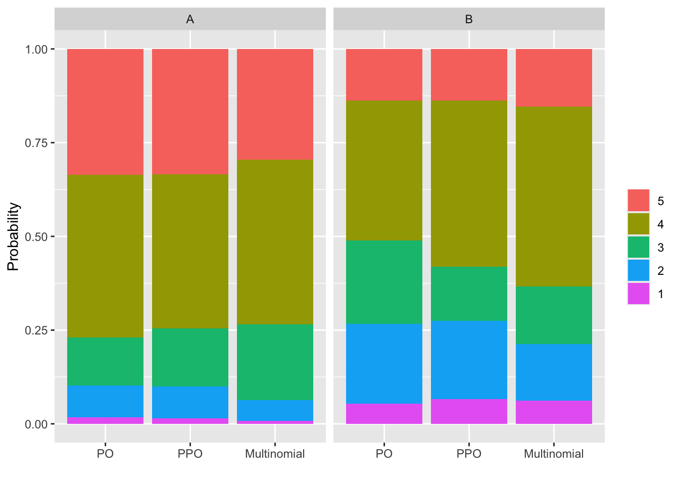
For all the covariate combinations evaluate predicted probabilities for all levels of Y using the PO model and the relaxed assumption models
Use the bootstrap to compute confidence intervals for the differences in predicted values between a PO model and a relaxed model. This will put the differences in the right context by accounting for uncertainties. This guards against over-emphasis of differences when the sample size does not support estimation, especially for the relaxed model with more parameters. Note that the same problem occurs when comparing predicted unadjusted probabilities to observed proportions, as observed proportions can be noisy.
Level 5 of y has only 5 patients so we combine it with level 6 for fitting the two relaxed models that depend on individual cell frequencies. Similarly, level 0 has only 6 patients, so we combine it with level 1. The PPO model is fitted with the VGAM R package, and the nonpo argument below signifies that the PO assumption is only being relaxed for the treatment effect. The multinomial model allows not only non-PO for trt but also for baseline. See here for impactPO source code.
                          PO     PPO    Multinomial
Deviance                  395.58 393.10 388.36
d.f.                       6      9     12
AIC                       407.58 411.10 412.36
p                         2      5      8
LR chi^2                  69.41  71.89  76.63
LR - p                    67.41  66.89  68.63
LR chi^2 test for PO             2.48   7.22
  d.f.                            3      6
  Pr(>chi^2)                     0.4792 0.3013
MCS R2                    0.374  0.385  0.404
MCS R2 adj                0.366  0.364  0.371
McFadden R2               0.149  0.155  0.165
McFadden R2 adj           0.141  0.133  0.130
Mean |difference| from PO        0.021  0.042

Covariate combination-specific mean |difference| in predicted probabilities

        method trt baseline Mean |difference|
1          PPO   A        4             0.010
2          PPO   B        4             0.033
11 Multinomial   A        4             0.032
21 Multinomial   B        4             0.052

Bootstrap 0.95 confidence intervals for differences in model predicted
probabilities based on 300 bootstraps


  trt baseline
1   A        4

PO - PPO probability estimates

           1      2      3      4      5
Lower -0.004 -0.017 -0.058 -0.055 -0.042
Upper  0.008  0.018  0.008  0.081  0.058

PO - Multinomial probability estimates

          1      2      3      4      5
Lower 0.002 -0.017 -0.152 -0.105 -0.037
Upper 0.020  0.071 -0.006  0.107  0.133

  trt baseline
2   B        4

PO - PPO probability estimates

           1      2      3      4      5
Lower -0.043 -0.077 -0.025 -0.191 -0.101
Upper  0.013  0.083  0.197  0.065  0.095

PO - Multinomial probability estimates

           1      2      3      4      5
Lower -0.050 -0.025 -0.051 -0.272 -0.143
Upper  0.035  0.147  0.194  0.041  0.095
Comparisons of the PO model fit with models that relax the PO assumption above can be summarized as follows.
By AIC, the model that is most likely to have the best cross-validation performance is the fully PO model (the lower the AIC the better)
There is no evidence for non-PO, either when judging against a model that relaxes the PO assumption for treatment (P=0.48) or against a multinomial logistic model that does not assume PO for any variables (P=0.30).
The McFadden adjusted \(R^2\) index, in line with AIC, indicates the best fit is from the PO model
The Maddala-Cox-Snell adjusted \(R^2\) indicates the PO model is competitive. See this for information about general adjusted \(R^2\) measures.
Nonparametric bootstrap percentile confidence intervals for the difference in predicted values between the PO model and one of the relaxed models take into account uncertainties and correlations of both sets of estimates. In all cases the confidence intervals are quite wide and include 0 (except for one case, where the lower confidence limit is 0.002), which is very much in line with apparent differences being clouded by overfitting (high number of parameters in non-PO models).
These assessments must be kept in mind when interpreting the inter-model agreement between probabilities of all levels of the ordinal outcome in the graphic that follows. According to AIC and adjusted \(R^2\), the estimates from the partial PO model and especially those from the multinomial model are overfitted. This is related to the issue that odds ratios computed from oversimplifying an ordinal response by dichotomizing it are noisy (also see the next to last section below).
AIC is essentially a forecast of what is likely to happen were the accuracy of two competing models be computed on a new dataset not used to fit the model. Had the observational study’s sample size been much larger, we could have randomly split the data into training and test samples and had a head-to-head comparison of the predictive accuracy of a PO model vs. a non-PO (multinomial or partial PO) model in the test sample. Non-PO models will be more unbiased but pay a significant price in terms of variance of estimates. The AIC and adjusted \(R^2\) analyses above suggest that the PO model will have lower mean squared errors of outcome probability estimates due to the strong reduction in variance (also see below).
Efficiency of Analyses Using Cutpoints
Clearly, the dependence of the proportional odds model on the assumption of proportionality can be over-stressed. Suppose that two different statisticians would cut the same three-point scale at different cut points. It is hard to see how anybody who could accept either dichotomy could object to the compromise answer produced by the proportional odds model. — Stephen Senn
Above I considered evidence in favor of making the PO assumption. Now consider the cost of not making the assumption. What is the efficiency of using a dichotomous endpoint? Efficiency can be captured by comparing the variance of an inefficient estimate to the variance of the most efficient estimate (which comes from the PO model by using the full information in all levels of the outcome variable). We don’t know the true variances of estimated treatment effects so instead use the estimated variances from fitted PO and binary logistic models.
Code
vtrt <-function(fit) vcov(fit)['trt=B', 'trt=B']vpo <-vtrt(f)w <-NULLfor(cutoff in1:6) { h <-lrm(y >= cutoff ~ trt + baseline, data=d) eff <- vpo /vtrt(h)# To discuss later: critical multiplicative error in OR cor <-exp(sqrt(vtrt(h) - vpo)) w <-rbind(w, data.frame(Cutoff=paste0('y≥', cutoff),Efficiency=round(eff, 2),`Sample Size Ratio`=round(1/eff, 1),`Critical OR Factor`=round(cor, 2),check.names=FALSE)) }w
Under PO the odds ratio from the PO model estimates the same quantity as the odds ratio from any dichotomization of the outcome. The relative efficiency of a dichotomized analysis is the variance of the most efficient (PO model) model’s log odds ratio for treatment divided by the variance of the log odds ratio from a binary logistic model using the dichotomization. The optimal cutoff (mainly due to being a middle value in the frequency distribution) is y≥4. For this dichotomization the efficiency is 0.56 (i.e., analyzing y≥4 vs. y is equivalent to discarding 44% of the sample) and the variance of the treatment log odds ratio is \(1.8 \times\) greater than the variance of the log odds ratio from the proportional odds model without binning. This means that the study would have to be \(1.8 \times\) larger to have the same power when dichotomizing the outcome as a smaller study that did not dichotomize it. Other dichotomizations result in even worse efficiency.
PO Model Results are Meaningful Even When PO is Violated
Overall Efficacy Assessment
Putting aside covariate adjustment, the PO model is equivalent to a Wilcoxon-Mann-Whitney two-sample rank-sum test statistic. The normalized Wilcoxon statistic (concordance probability; also called probability index) is to within a high degree of approximation a simple function of the estimated odds ratio from a PO model fit. Over a wide variety of datasets satisfying and violating PO, the \(R^2\) for predicting the log odds ratio from the logit of the scaled Wilcoxon statistic is 0.996, and the mean absolute error in predicting the concordance probability from the log odds ratio is 0.002. See Violation of Proportional Odds is Not Fatal and If You Like the Wilcoxon Test You Must Like the Proportional Odds Model.
Let’s compare the actual Wilcoxon concordance probability with the concordance probability estimated from the odds ratio without covariate adjustment, \(\frac{\mathrm{OR}^{0.65}}{1 + \mathrm{OR}^{0.65}}\).
Code
w <-wilcox.test(y ~ trt, data=d)w
    Wilcoxon rank sum test with continuity correction

data:  y by trt
W = 2881, p-value = 0.04395
alternative hypothesis: true location shift is not equal to 0
Code
W <- w$statisticconcord <- W /prod(table(d$trt))
Code
u <-lrm(y ~ trt, data=d)u
Logistic Regression Model
lrm(formula = y ~ trt, data = d)
Frequencies of Responses
 0  1  2  3  4  5  6
 6 19 39 24 40  5 15
Model Likelihood
Ratio Test
Discrimination
Indexes
Rank Discrim.
Indexes
Obs 148
LR χ2 4.18
R2 0.029
C 0.555
max |∂log L/∂β| 2×10⁻⁷
d.f. 1
R21,148 0.021
Dxy 0.110
Pr(>χ2) 0.0409
R21,141.3 0.022
γ 0.247
Brier 0.240
τa 0.088
β
S.E.
Wald Z
Pr(>|Z|)
y≥1
3.4217
0.4390
7.79
<0.0001
y≥2
1.8302
0.2524
7.25
<0.0001
y≥3
0.4742
0.1948
2.43
0.0149
y≥4
-0.1890
0.1929
-0.98
0.3272
y≥5
-1.6691
0.2561
-6.52
<0.0001
y≥6
-1.9983
0.2858
-6.99
<0.0001
trt=B
-0.6456
0.3174
-2.03
0.0420
Note that the \(C\) statistic in the above table handles ties differently than the concordance probability we are interested in here.
Code
or <-exp(-coef(u)['trt=B'])cat('Concordance probability from Wilcoxon statistic: ', concord, '\n','Concordance probability estimated from OR: ', or ^0.65/ (1+ or ^0.65), '\n', sep='')
Concordance probability from Wilcoxon statistic: 0.6002083
Concordance probability estimated from OR: 0.6033931
In the absence of adjustment covariates, the treatment odds ratio estimate from a PO model is essentially the Wilcoxon statistic whether or not PO holds. Many statisticians are comfortable with using the Wilcoxon statistic for judging which treatment is better overall, e.g., which treatment tends to move responses towards the favorable end of the scale. So one can seldom go wrong in using the PO model to judge which treatment is better, even when PO does not hold.
Simulation Study of Effect of Adjusting for a Highly Non-PO Covariate
What if the treatment operates in PO but an important covariate strongly violates its PO assumption? Let’s find out by simulating a specific departure from PO for a binary covariate. For a discrete ordinal outcome with levels 0,1,…,6 let the intercepts corresponding to \(Y=1, ..., 6\) be \(\alpha = [4.4, 2.6, 0.7, -0.2, -2, -2.4]\). Let the true treatment effect be \(\beta=-1.0\). The simulated covariate \(X\) is binary with a prevalence of \(\frac{1}{2}\). The true effect of \(X\) is to have an OR of 3.0 on \(Y\geq 1\), \(Y\geq 2\), \(Y\geq 3\) but to have an OR of \(\frac{1}{3}\) on \(Y\geq 4\), \(Y\geq 5\) and \(Y=6\). So the initial regression coefficient for \(X\) is \(\log(3)\) and the additional effect of \(X\) on \(Y\geq y\) once \(y\) crosses to 4 and above is a decrement in its prevailing log odds by \(2\log(3)\). So here is our model to simulate from:
\[\Pr(Y \geq y | \mathrm{trt}, X) = \mathrm{expit}(\alpha_{y} - [\mathrm{trt=B}] + \log(3) X -2\log(3) X [y \geq 4])\]
Over simulations compare these three estimates and their standard error:
unadjusted treatment effect
treatment effect adjusted for covariate assuming both treatment and covariate act in PO
treatment effect adjusted for covariate assuming treatment is PO but allowing the covariate to be arbitrarily non-PO
To test the simulation, simulate a very large sample size of n=50,000 and examine the coefficient estimates from the correct partial PO model and from two other models.
Code
sim <-function(beta, n, nsim=100) { tx <-c(rep(0, n/2), rep(1, n/2)) x <-c(rep(0, n/4), rep(1, n/4), rep(0, n/4), rep(1, n/4))# Construct a matrix of logits of cumulative probabilities L <-matrix(alpha, nrow=n, ncol=6, byrow=TRUE) L[tx ==1,] <- L[tx ==1, ] + beta L[x ==1, ] <- L[x ==1, ] +log(3) L[x ==1, 4:6] <- L[x ==1, 4:6] -2*log(3) P <-plogis(L) # cumulative probs P <-cbind(1, P) -cbind(P, 0) # cell probs (each row sums to 1.0) b <- v <- pv <-matrix(NA, nrow=nsim, ncol=3)colnames(b) <-colnames(v) <-colnames(pv) <-c('PPO', 'PO', 'No X') y <-integer(n) a <-'tx' msim <-0for(i in1: nsim) {for(j in1: n) y[j] <-sample(0:6, 1, prob=P[j, ]) f <-try(vglm(y ~ tx + x, cumulative(reverse=TRUE, parallel=FALSE~ x)))if(inherits(f, 'try-error')) next msim <- msim +1 g <-lrm(y ~ tx + x) h <-lrm(y ~ tx) co <-c(coef(f)[a], coef(g)[a], coef(h)[a]) vs <-c(vcov(f)[a,a], vcov(g)[a,a], vcov(h)[a,a]) b[msim, ] <- co v[msim, ] <- vs pv[msim, ] <-2*pnorm(-abs(co /sqrt(vs))) } b <- b [1:msim,, drop=FALSE] v <- v [1:msim,, drop=FALSE] pv <- pv[1:msim,, drop=FALSE] bbar <-apply(b, 2, mean) bmed <-apply(b, 2, median) bse <-sqrt(apply(v, 2, mean)) bsemed <-sqrt(apply(v, 2, median)) sd <-if(msim <2) rep(NA, 3) elsesqrt(diag(cov(b))) pow <-if(nsim <2) rep(NA, 3) elseapply(pv, 2, function(x) mean(x <0.05))list(summary=cbind('Mean beta'= bbar,'Median beta'= bmed,'Sqrt mean estimated var'= bse,'Median estimated SE'= bsemed,'Empirical SD'= sd,'Power'= pow),sims=list(beta=b, variance=v, p=pv),nsim=msim)}require(VGAM)alpha <-c(4.4, 2.6, 0.7, -0.2, -2, -2.4)set.seed(1)si <-sim(beta=-1, 50000, 1)round(si$summary, 4)
     Mean beta Median beta Sqrt mean estimated var Median estimated SE
PPO    -0.9832     -0.9832                  0.0176              0.0176
PO     -0.9271     -0.9271                  0.0168              0.0168
No X   -0.9280     -0.9280                  0.0168              0.0168
     Empirical SD Power
PPO            NA    NA
PO             NA    NA
No X           NA    NA
With n=50,000 extreme non-PO in the binary covariate hardly affected the estimated treatment and its standard error, and did not affect the ratio of the coefficient estimate to its standard error. Non-PO in \(X\) does effect the intercepts which has an implication in estimating absolute effects (unlike the treatment OR). But by examining the intercepts when the covariate is omitted entirely one can see that the problems with the intercepts when PO is forced are no worse than just ignoring the covariate altogether (not shown here).
Now simulate 2000 trials with n=300 and study how the various models perform.
Code
set.seed(7)fi <-'~/data/sim/simtx.rds'if(file.exists(fi)) simr <-readRDS(fi) else { s <-sim(-1, 300, 2000) s0 <-sim( 0, 300, 2000) # also simulate under the null simr <-list(s=s, s0=s0)saveRDS(simr, fi)}cat('Convergence in', simr$s$nsim, 'simulations\n\n')
Convergence in 1947 simulations
Code
kab(round(simr$s$summary, 4))
Mean beta
Median beta
Sqrt mean estimated var
Median estimated SE
Empirical SD
Power
PPO
-1.0157
-1.0100
0.2273
0.2281
0.2340
0.9979
PO
-0.9609
-0.9565
0.2189
0.2184
0.2227
0.9974
No X
-0.9599
-0.9556
0.2188
0.2183
0.2227
0.9974
The second line of the summary shows what to expect when fitting a PO model in the presence of severe non-PO for an important covariate. The mean estimated treatment effect is the same as not adjusting for the covariate and so is its estimated standard error. Both are close to the estimate from the proper model—the partial PO model that allows for different effects of \(X\) over the categories of \(Y\). And for all three models the standard error of the treatment effect estimated from that model’s information matrix is very accurate as judged by the closeness to the empirical SD of the simulated regression coefficient estimates.
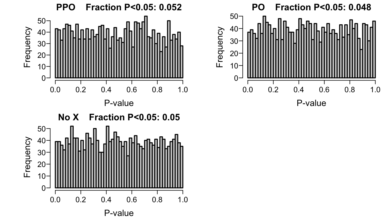
Check simulations under the null, i.e., with \(\beta=0\) for treatment. Look at the distribution of p-values for the three model’s treatment 2-sided Wald tests (which should be uniform), and the empirical \(\alpha\), the fraction of Wald p-values \(< 0.05\).
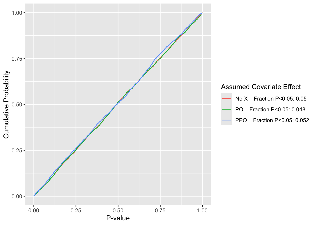
Empirical cumulative distributions of p-values from Wald tests of the treatment effect under the null \(\beta=0\), with simulation estimates of \(\alpha\) for three models for a strong covariate \(X\)
\(\alpha\) under the improper (with respect to \(X\)) PO model is just under that of the model ignoring \(X\), which is estimated to be at the nominal 0.05. The estimated \(\alpha\) for the appropriate partial PO model is just over 0.05.
Using the PO Model to Estimate the Treatment Effect for a Specific Y Cutoff
Just as in the case where one thinks that a sex by treatment interaction may be present, actually estimating such an interaction effect can make treatment estimates worse for both sexes in small samples even when the interaction is truly present. This is because estimating an unknown quantity well requires both minimal bias and good precision (low variance), and adding a parameter to the model increases variance (one must estimate both the main effect and the interaction, equivalent to estimating separate treatment effects for females and males). The probability that an estimate is within a given tolerance of the true value is closely related to the mean squared error (MSE) of the estimator. MSE equals variance plus the square of bias. Bias is the systematic error that can result from model misspecification, e.g., fitting a common OR (assuming PO) when the treatment OR needs to vary for some levels of Y (non-PO).
A log odds ratio estimate for a specific cutoff Y≥y derived from a model that dichotomized the raw data at y will tend to be unbiased for estimating that specific log odds ratio. Suppose the log OR has variance \(u\). The MSE of the log OR estimate is \(u\) since the bias is approximately zero. Now consider estimating the common OR in a PO model and using that to estimate the OR for Y≥y. Suppose that common log OR has variance \(v\) and bias \(b\) (\(b\) is a weighted log OR the PO model estimates minus the true log OR for Y≥y) so that MSE of the log OR for the PO model is \(v + b^2\). The multiplicative bias (fold-change bias) is \(e^b\). How large must this multiplicative bias in the OR estimate be (i.e., how much non-PO needs to exist) before the tailored model for Y≥y has lower mean squared error (on the log scale) than the less-well-fitting PO model? By comparing the two MSEs of \(u\) and \(v + b^2\) we find that the critical multiplicative error in the OR is \(\exp(\sqrt{u - v})\).
For the dataset we have been analyzing, the critical fold change in OR is tabulated in the table above under the column Critical OR Factor. For example, for the lowest cutoff this factor is 2.33. This is interpreted as saying that an ill-fitting PO model would still break even with a tailored well-fitting model (one that suffers from having higher variance of \(\hat{\beta}\) due to not breaking ties in Y) in terms of the chance of having the OR estimate close to the true OR, as long as the true combined estimand PO OR is not more than a factor of 2.33 away from the true OR for Y≥1. For example, if the OR that the PO model is estimating is 2, this estimate would be equal in accuracy to a tailored sure-to-fit estimate if the true PO is 4.66, and would be better than the tailored estimate if the true OR is less than 4.66.
Looking over all possible cutoffs, a typical OR critical fold change is 1.5. Loosely speaking if ORs for two different cutoffs have a ratio less than 1.5 and greater than 1/1.5 the PO model will provide a more accurate treatment OR for a specific cutoff than will an analysis built around estimating the OR only for that cutoff. As the sample size grows, the critical multiplicative change in OR will fall. This leads to the next section.
A Continuous Solution
Instead of assessing the adequacy of the PO assumption, hoping that the data contain enough information to discern whether a PO model is adequate and then making a binary decision (PO or non-PO model), a far better approach is to allow for non-PO to the extent that the current sample size allows. By scaling the amount of non-PO allowed, resulting in a reasonable amount of borrowing of information across categories of Y, one can achieve a good mean squared error of an effect estimator. This can be achieved using a Bayesian partial proportional odds model with a skeptical prior distribution for the parameters representing departures from the PO assumption. As the sample size increases, the prior wears off, and the PO assumption is progressively relaxed. All uncertainties are accounted for, and the analyst need not make a PO/non-PO choice. This is implemented in the R rmsb package blrm function. See this for discussion of using this approach for a formal analysis studying to what extent a treatment effects one part of the outcome scale differently than it affects other parts.
To get a feeling for how the degree of skepticism of the prior for the departure from PO relates to the MSE of a treatment effect, we choose normal distributions with mean 0 and various variances, compute penalized maximum likelihood estimates (PMLEs). These PMLEs are computed by forming the prior and the likelihood and having the Bayesian procedure optimize the penalized likelihood and not do posterior sampling, to save time. Note that the reciprocal of the variance of the prior is the penalty parameter \(\lambda\) in PMLE (ridge regression).
Going along with examples shown here, consider a 3-level response variable Y=0,1,2 and use the following partial PO model for the two-group problem without covariates. Here treatment is coded x=0 for control, x=1 for active treatment.
\[\Pr(Y \geq j | x) = \mathrm{expit}(\alpha_{y} + x\beta + \tau x[y=2])\] When \(\tau=0\) PO holds. \(\tau\) is the additional treatment effect on \(Y=2\).
Consider true probabilities for Y=0,1,2 when x=0 to be the vector p0 in the code below, and when x=1 to be the vector p1. These vectors are not in proportional odds. Draw samples of size 100 from each of these two multinomial distributions, with half having x=0 and half having x=1. Compute the PMLE for various prior distributions for \(\tau\) that are normal with mean 0 and with SD varying over 0.001 (virtually assuming PO), 0.1, 0.5, 0.75, 1, 1.5, 2, 4 (almost fully trusting the partial PO model fit, with very little discounting of \(\tau\)). When the prior SD for the amount of non-PO \(\tau\) is 0.5, this translates to a prior probability of 0.02275 that \(\tau > 1\) and the same for \(\tau < -1\).
True model parameters are solved for using the following:
require(rmsb)p0 <-c(.4, .2, .4)p1 <-c(.3, .1, .6)lors <-c('log OR for Y>=1'=qlogis(0.7) -qlogis(0.6),'log OR for Y=2'=qlogis(0.6) -qlogis(0.4))alpha1 <-qlogis(0.6)alpha2 <-qlogis(0.4)beta <-qlogis(0.7) - alpha1tau <-qlogis(0.6) - alpha2 - betac(alpha1=alpha1, alpha2=alpha2, beta=beta, tau=tau)
    alpha1     alpha2       beta        tau
 0.4054651 -0.4054651  0.4418328  0.3690975
Let’s generate a very large (n=20,000) patient dataset to check the above calculations by getting unpenalized MLEs.
Code
m <-10000# observations per treatmentm0 <- p0 * m # from proportions to frequenciesm1 <- p1 * mx <-c(rep(0, m), rep(1, m))y0 <-c(rep(0, m0[1]), rep(1, m0[2]), rep(2, m0[3]))y1 <-c(rep(0, m1[1]), rep(1, m1[2]), rep(2, m1[3]))y <-c(y0, y1)table(x, y)
   y
x      0    1    2
  0 4000 2000 4000
  1 3000 1000 6000
Code
# Create a contrast so that we can put a prior on the PO effect of xg <-function(y) y ==2options(rmsb.backend='cmdstan', mc.cores=4)cmdstanr::set_cmdstan_path(cmdstan.loc)f <-blrm(y ~ x, ~x, cppo=g, method='opt')
Initial log joint probability = -21971.6
    Iter      log prob        ||dx||      ||grad||       alpha      alpha0  # evals  Notes
      32        -19528    0.00770102      0.271742      0.7175      0.7175       38
Optimization terminated normally:
  Convergence detected: relative gradient magnitude is below tolerance
Finished in  0.3 seconds.
Code
coef(f)
      y>=1       y>=2          x   x x f(y)
 0.4055323 -0.4053735  0.4418074  0.3690617
Code
# Also check estimates when a small prior SD is put on taunpc <-list(sd=0.0001, c1=list(x=1), c2=list(x=0),contrast=expression(c1 - c2))f <-blrm(y ~ x, ~x, cppo=g, npcontrast=npc, method='opt')
Initial log joint probability = -21963.3
    Iter      log prob        ||dx||      ||grad||       alpha      alpha0  # evals  Notes
      23      -19666.9     0.0250004      0.328862      0.9056      0.9056       27
Optimization terminated normally:
  Convergence detected: relative gradient magnitude is below tolerance
Finished in  0.1 seconds.
Code
coef(f) # note PMLE of tau is almost zero
         y>=1          y>=2             x      x x f(y)
 3.176969e-01 -3.177318e-01  6.600601e-01  7.589660e-06
Code
# Compare with a PO modelcoef(lrm(y ~ x))
      y>=1       y>=2          x
 0.3176995 -0.3176995  0.6600599
Let’s also simulate for 1000 in each group the variance of the difference in log ORs.
Code
m <-1000x <-c(rep(0, m), rep(1, m))nsim <-5000set.seed(2)lg <-function(y) qlogis(mean(y))dlor <-numeric(nsim)for(i in1: nsim) { y0 <-sample(0:2, m, replace=TRUE, prob=p0) y1 <-sample(0:2, m, replace=TRUE, prob=p1) dlor[i] <-lg(y1 ==2) -lg(y0 ==2) - (lg(y1 >=1) -lg(y0 >=1))}mean(dlor)
[1] 0.368478
Code
v1000 <-var(dlor)v100 <- v1000 * (1000/100)cat('Variance of difference in log(OR): 1000 per group:', v1000, ' 100 per group:', v100, '\n')
Variance of difference in log(OR): 1000 per group: 0.004667525 100 per group: 0.04667525
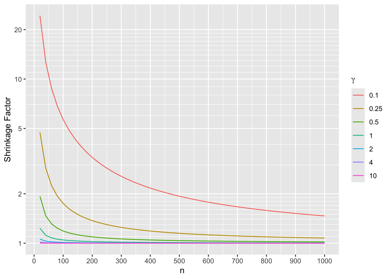
For a sample containing n subjects per treatment arm, the variance of the difference in the two log ORs (i.e., the amount of deviation from PO) is approximately \(\sigma^{2} = \frac{4.668}{n}\). An approximate way to think of the effect of a skeptical prior on the difference in log ORs \(\tau\) is to assume that \(\hat{\tau}\) has a normal distribution with mean \(\tau\) and variance \(\sigma^2\). When the prior for \(\tau\) has mean 0 and variance \(\gamma^2\), the posterior mean for \(\tau\) is \(\frac{\hat{\tau}}{1 + \frac{\sigma^2}{\gamma^2}}\) The denominator is the shrinkage factor \(s\). Study how \(s\) varies with \(\gamma^2\) and \(n\).
One can see for example that when the prior SD for \(\tau\) is \(\gamma=1\) the prior causes an estimate of \(\tau\) to shrink only by only about a factor of 1.25 even for very small sample sizes. By the time there are 200 patients per treatment arm the shrinkage towards PO is not noticeable.
The following simulations for 100 patients per arm provide more accurate estimates because formal PMLE is used and the data likelihood is not assumed to be Gaussian. In addition to quantifying the effect of shrinkage caused by different \(\gamma\) (prior SD of \(\tau\)), we compute the root mean squared errors for estimating log(OR) for \(Y\geq 1\) and for \(Y=2\).
Code
m <-100x <-c(rep(0, m), rep(1, m))nsim <-500sds <-c(.0001, 0.1, 0.5, 0.75, 1, 1.5, 2, 4, 10, 50)lsd <-length(sds)gam <-if(ishtml) 'γ'else'$\\gamma$'if(file.exists('Rsimsd.rds')) R <-readRDS('Rsimsd.rds') else { R <-array(NA, c(nsim, lsd, 2),dimnames=list(NULL, paste0(gam, '=', sds),c('Y>=1', 'Y=2')))set.seed(3)for(i in1: nsim) { y0 <-sample(0:2, m, replace=TRUE, prob=p0) y1 <-sample(0:2, m, replace=TRUE, prob=p1) y <-c(y0, y1)for(j in1: lsd[1]) { npc <-list(sd=sds[j], c1=list(x=1), c2=list(x=0),contrast=expression(c1 - c2)) f <-blrm(y ~ x, ~ x, cppo=g, npcontrast=npc, method='opt') k <-coef(f)# save the two treatment log ORs (for Y>=1 and for Y=2) R[i, j, 1:2] <-c(k['x'], k['x'] + k['x x f(y)']) } }saveRDS(R, 'Rsimsd.rds')}# For each prior SD compute the two mean log ORs and compare# truthcat('True values:\n')
True values:
Code
lors
log OR for Y>=1  log OR for Y=2
      0.4418328       0.8109302
In a mixed Bayesian/frequentist sense (computing MSE of a posterior mean), the optimum MSE in estimating the two treatment effects (log ORs) was obtained at \(\gamma=2\). The observed shrinkage factors do not track very well with the approximate ones derived earlier. A better approximation is needed.
Further Reading
See a similar case study in RMS Section 13.3.5. In that example, the sample size is larger and PO is clearly violated.
Computing Environment
 R version 4.3.2 (2023-10-31)
 Platform: aarch64-apple-darwin20 (64-bit)
 Running under: macOS Sonoma 14.3.1

 Matrix products: default
 BLAS:   /Library/Frameworks/R.framework/Versions/4.3-arm64/Resources/lib/libRblas.0.dylib
 LAPACK: /Library/Frameworks/R.framework/Versions/4.3-arm64/Resources/lib/libRlapack.dylib;  LAPACK version 3.11.0

 attached base packages:
 [1] splines   stats4    stats     graphics  grDevices utils     datasets
 [8] methods   base

 other attached packages:
 [1] rmsb_1.1-0    VGAM_1.1-10   ggplot2_3.5.0 rms_6.8-0     Hmisc_5.1-2
To cite R in publications use:
R Core Team (2023).
R: A Language and Environment for Statistical Computing.
R Foundation for Statistical Computing, Vienna, Austria.
https://www.R-project.org/.
---title: Assessing the Proportional Odds Assumption and Its Impactauthor: - name: Frank Harrell affiliation: Department of Biostatistics<br>Vanderbilt University School of Medicine url: https://hbiostat.orgdate: 2022-03-09categories: [2022, accuracy-score, dichotomization, endpoints, ordinal]description: "This article demonstrates how the proportional odds (PO) assumption and its impact can be assessed. General robustness to non-PO on either a main variable of interest or on an adjustment covariate are exemplified. Advantages of a continuous Bayesian blend of PO and non-PO are also discussed."---```{r setup, include=FALSE}require(rms)require(ggplot2)knitrSet(lang='quarto')source('~/rr/rmarkdown/qbookfun.r')options(prType=if(ishtml) 'html'else'latex')options(omitlatexcom=TRUE)# keeps Pandoc from messing up generated LaTeX commentsggp <- ggplotlyr # ggplotlyr is in Hmisc# Gets around a bug in tooltip construction with ggplotlypr <- markupSpecs$markdown$prkab <- knitr::kable```<a href="https://atlas.mindmup.com/vbiostat/po"><img src="pomap.png" width="100%" alt=""></a>`r disccom('rms-ordinal-logistic-regression')`# IntroductionReviewers who do not seem to worry about the proportional hazards assumption in a Cox model or the equal variance assumption in a $t$-test seem to worry a good deal about the proportional odds (PO) assumption in a semiparametric ordinal logistic regression model. This in spite of the fact that proportional hazards and equal variance in other models are exact analogies to the PO assumption. Furthermore, when there is no covariate adjustment, the PO model is equivalent to the Wilcoxon test, and reviewers do not typically criticize the Wilcoxon test or realize that it has optimum power only under the PO assumption. [[Comments](https://hbiostat.org/comment.html)]{.aside}The purpose of this report is to (1) demonstrate examinations of the PO assumption for a treatment effect in a two-treatment observational comparison, and (2) discuss various issues around PO model analysis and alternative analyses using cutpoints on the outcome variable. It is shown that exercises such as comparing predicted vs. observed values can be misleading when the sample size is not very large.# DatasetThe dataset, taken from a real observational study, consists of a 7-level ordinal outcome variable `y` having values 0-6, a treatment variable `trt`, and a strong baseline variable `baseline` defined by a disease scale that is related to `y` but with more resolution. This is a dominating covariate, and failure to adjust for it will result in a weaker treatment comparison. `trt` levels are A and B, with 48 patients given treatment B and 100 given treatment A.```{r desc,results='asis'}getHdata(txpo)d <- txpodd <-datadist(d); options(datadist='dd')if(ishtml) html(describe(d)) elselatex(describe(d), file='')with(d, pr(obj=table(trt, y)))```# Proportional Odds Model```{r mod1,results='asis'}f <-lrm(y ~ trt + baseline, data=d)fsummary(f)anova(f)```# Volatility of ORs Using Different CutoffsEven when the data generating mechanism is exactly proportional odds for treatment, different cutoffs of the response variable Y can lead to much different ORs when the sample size is not in the thousands. This is just the play of chance (sampling variation). To illustrate this point, consider the observed proportions of Y for `trt=A` as population probabilities for A. Apply an odds ratio of 0.3 to get the population distribution of Y for treated patients. For 10 simulated trials, sample from these two multinomial distributions and compute sample ORs for all Y cutoffs. ```{r sim}p <-table(d$y[d$trt =='A'])p <- p /sum(p)p # probabilities for SOCset.seed(1)round(simPOcuts(n=210, odds.ratio=0.3, p=p), 2)```See [here](https://github.com/harrelfe/Hmisc/blob/master/R/popower.s) for `simPOcuts` source code.# Examining the PO AssumptionFor discrete Y we are interested in checking the impact ofthe PO assumption on predicted probabilities for all of the Ycategories, while also allowing for covariate adjustment. This can bedone using the following steps:* Select a set of covariate settings over which to evaluate accuracy of predictions* Vary at least one of the predictors, i.e., the one for which you want to assess the impact of the PO assumption* Fit a PO model the usual way* Fit models that relaxes the PO assumption + to relax the PO assumption for all predictors fit a multinomial logistic model + to relax the PO assumption for a subset of predictors fit a partial PO (PPO) model* For all the covariate combinations evaluate predicted probabilities for all levels of Y using the PO model and the relaxed assumption models* Use the bootstrap to compute confidence intervals for the differences in predicted values between a PO model and a relaxed model. This will put the differences in the right context by accounting for uncertainties. This guards against over-emphasis of differences when the sample size does not support estimation, especially for the relaxed model with more parameters. Note that the same problem occurs when comparing predicted unadjusted probabilities to observed proportions, as observed proportions can be noisy.Level 5 of `y` has only 5 patients so we combine it with level 6 for fitting the two relaxed models that depend on individual cell frequencies. Similarly, level 0 has only 6 patients, so we combine it with level 1. The PPO model is fitted with the `VGAM` R package, and the `nonpo` argument below signifies that the PO assumption is only being relaxed for the treatment effect. The multinomial model allows not only non-PO for `trt` but also for `baseline`. See [here](https://github.com/harrelfe/rms/blob/master/R/impactPO.r) for `impactPO` source code.```{r impactpo}nd <-data.frame(trt=levels(d$trt), baseline=4)d$y5 <-with(d, pmin(pmax(y, 1), 5))w <-impactPO(y5 ~ trt + baseline, nonpo =~ trt,data=d, newdata=nd, B=300)w```Comparisons of the PO model fit with models that relax the PO assumption above can be summarized as follows.* By AIC, the model that is most likely to have the best cross-validation performance is the fully PO model (the lower the AIC the better)* There is no evidence for non-PO, either when judging against a model that relaxes the PO assumption for treatment (P=0.48) or against a multinomial logistic model that does not assume PO for any variables (P=0.30).* The McFadden adjusted $R^2$ index, in line with AIC, indicates the best fit is from the PO model* The Maddala-Cox-Snell adjusted $R^2$ indicates the PO model is competitive. See [this](https://hbiostat.org/bib/r2.html) for information about general adjusted $R^2$ measures.* Nonparametric bootstrap percentile confidence intervals for the difference in predicted values between the PO model and one of the relaxed models take into account uncertainties and correlations of both sets of estimates. In all cases the confidence intervals are quite wide and include 0 (except for one case, where the lower confidence limit is 0.002), which is very much in line with apparent differences being clouded by overfitting (high number of parameters in non-PO models).These assessments must be kept in mind when interpreting the inter-model agreement between probabilities of all levels of the ordinal outcome in the graphic that follows. According to AIC and adjusted $R^2$, the estimates from the partial PO model and especially those from the multinomial model are overfitted. This is related to the issue that odds ratios computed from oversimplifying an ordinal response by dichotomizing it are noisy (also see the next to last section below).```{r plimpactpo}revo <-function(z) { z <-as.factor(z)factor(z, levels=rev(levels(as.factor(z))))}ggplot(w$estimates, aes(x=method, y=Probability, fill=revo(y))) +facet_wrap(~ trt) +geom_col() +xlab('') +guides(fill=guide_legend(title=''))```AIC is essentially a forecast of what is likely to happen were the accuracy of two competing models be computed on a new dataset not used to fit the model. Had the observational study's sample size been much larger, we could have randomly split the data into training and test samples and had a head-to-head comparison of the predictive accuracy of a PO model vs. a non-PO (multinomial or partial PO) model in the test sample. Non-PO models will be more unbiased but pay a significant price in terms of variance of estimates. The AIC and adjusted $R^2$ analyses above suggest that the PO model will have lower mean squared errors of outcome probability estimates due to the strong reduction in variance (also see below).# Efficiency of Analyses Using Cutpoints::: {.column-margin}Clearly, the dependence of the proportional odds model on the assumption of proportionality can be over-stressed. Suppose that two different statisticians would cut the same three-point scale at different cut points. It is hard to see how anybody who could accept either dichotomy could object to the compromise answer produced by the proportional odds model. — [Stephen Senn](https://onlinelibrary.wiley.com/doi/abs/10.1002/sim.3603):::Above I considered evidence in favor of making the PO assumption. Now consider the cost of **not** making the assumption. What is the efficiency of using a dichotomous endpoint? Efficiency can be captured by comparing the variance of an inefficient estimate to the variance of the most efficient estimate (which comes from the PO model by using the full information in all levels of the outcome variable). We don't know the true variances of estimated treatment effects so instead use the estimated variances from fitted PO and binary logistic models.```{r eff}vtrt <-function(fit) vcov(fit)['trt=B', 'trt=B']vpo <-vtrt(f)w <-NULLfor(cutoff in1:6) { h <-lrm(y >= cutoff ~ trt + baseline, data=d) eff <- vpo /vtrt(h)# To discuss later: critical multiplicative error in OR cor <-exp(sqrt(vtrt(h) - vpo)) w <-rbind(w, data.frame(Cutoff=paste0('y≥', cutoff),Efficiency=round(eff, 2),`Sample Size Ratio`=round(1/eff, 1),`Critical OR Factor`=round(cor, 2),check.names=FALSE)) }w```The last column is discussed in a later section.Under PO the odds ratio from the PO model estimates the same quantity as the odds ratio from any dichotomization of the outcome. The relative efficiency of a dichotomized analysis is the variance of the most efficient (PO model) model's log odds ratio for treatment divided by the variance of the log odds ratio from a binary logistic model using the dichotomization.The optimal cutoff (mainly due to being a middle value in the frequency distribution) is y≥4. For this dichotomization the efficiency is 0.56 (i.e., analyzing y≥4 vs. y is equivalent to discarding 44% of the sample) and the variance of the treatment log odds ratio is $1.8 \times$ greater than the variance of the log odds ratio from the proportional odds model without binning. This means that the study would have to be $1.8 \times$ larger to have the same power when dichotomizing the outcome as a smaller study that did not dichotomize it. Other dichotomizations result in even worse efficiency.For more examples of relative efficiencies for various outcome configurations see [Information Gain From Using Ordinal Instead of Binary Outcomes](../ordinal-info).# PO Model Results are Meaningful Even When PO is Violated## Overall Efficacy AssessmentPutting aside covariate adjustment, the PO model is equivalent to a Wilcoxon-Mann-Whitney two-sample rank-sum test statistic. The normalized Wilcoxon statistic (concordance probability; also called probability index) is to within a high degree of approximation a simple function of the estimated odds ratio from a PO model fit. Over a wide variety of datasets satisfying and violating PO, the $R^2$ for predicting the log odds ratio from the logit of the scaled Wilcoxon statistic is 0.996, and the mean absolute error in predicting the concordance probability from the log odds ratio is 0.002. See [Violation of Proportional Odds is Not Fatal](../po) and [If You Like the Wilcoxon Test You Must Like the Proportional Odds Model](../wpo).Let's compare the actual Wilcoxon concordance probability with the concordance probability estimated from the odds ratio without covariate adjustment, $\frac{\mathrm{OR}^{0.65}}{1 + \mathrm{OR}^{0.65}}$.```{r wilcox}w <-wilcox.test(y ~ trt, data=d)wW <- w$statisticconcord <- W /prod(table(d$trt))``````{r wilcox2,results='asis'}u <-lrm(y ~ trt, data=d)u```Note that the $C$ statistic in the above table handles ties differently than the concordance probability we are interested in here.```{r wilcox3}or <-exp(-coef(u)['trt=B'])cat('Concordance probability from Wilcoxon statistic: ', concord, '\n','Concordance probability estimated from OR: ', or ^0.65/ (1+ or ^0.65), '\n', sep='')```In the absence of adjustment covariates, the treatment odds ratio estimate from a PO model **is** essentially the Wilcoxon statistic whether or not PO holds. Many statisticians are comfortable with using the Wilcoxon statistic for judging which treatment is better overall, e.g., which treatment tends to move responses towards the favorable end of the scale. So one can seldom go wrong in using the PO model to judge which treatment is better, even when PO does not hold.## Simulation Study of Effect of Adjusting for a Highly Non-PO CovariateWhat if the treatment operates in PO but an important covariate strongly violates its PO assumption? Let's find out by simulating a specific departure from PO for a binary covariate. For a discrete ordinal outcome with levels 0,1,...,6 let the intercepts corresponding to $Y=1, ..., 6$ be $\alpha = [4.4, 2.6, 0.7, -0.2, -2, -2.4]$. Let the true treatment effect be $\beta=-1.0$. The simulated covariate $X$ is binary with a prevalence of $\frac{1}{2}$. The true effect of $X$ is to have an OR of 3.0 on $Y\geq 1$, $Y\geq 2$, $Y\geq 3$ but to have an OR of $\frac{1}{3}$ on $Y\geq 4$, $Y\geq 5$ and $Y=6$. So the initial regression coefficient for $X$ is $\log(3)$ and the additional effect of $X$ on $Y\geq y$ once $y$ crosses to 4 and above is a decrement in its prevailing log odds by $2\log(3)$. So here is our model to simulate from:$$\Pr(Y \geq y | \mathrm{trt}, X) = \mathrm{expit}(\alpha_{y} - [\mathrm{trt=B}] + \log(3) X -2\log(3) X [y \geq 4])$$Over simulations compare these three estimates and their standard error:* unadjusted treatment effect* treatment effect adjusted for covariate assuming both treatment and covariate act in PO* treatment effect adjusted for covariate assuming treatment is PO but allowing the covariate to be arbitrarily non-POTo test the simulation, simulate a very large sample size of n=50,000 and examine the coefficient estimates from the correct partial PO model and from two other models.```{r simtry}sim <-function(beta, n, nsim=100) { tx <-c(rep(0, n/2), rep(1, n/2)) x <-c(rep(0, n/4), rep(1, n/4), rep(0, n/4), rep(1, n/4))# Construct a matrix of logits of cumulative probabilities L <-matrix(alpha, nrow=n, ncol=6, byrow=TRUE) L[tx ==1,] <- L[tx ==1, ] + beta L[x ==1, ] <- L[x ==1, ] +log(3) L[x ==1, 4:6] <- L[x ==1, 4:6] -2*log(3) P <-plogis(L) # cumulative probs P <-cbind(1, P) -cbind(P, 0) # cell probs (each row sums to 1.0) b <- v <- pv <-matrix(NA, nrow=nsim, ncol=3)colnames(b) <-colnames(v) <-colnames(pv) <-c('PPO', 'PO', 'No X') y <-integer(n) a <-'tx' msim <-0for(i in1: nsim) {for(j in1: n) y[j] <-sample(0:6, 1, prob=P[j, ]) f <-try(vglm(y ~ tx + x, cumulative(reverse=TRUE, parallel=FALSE~ x)))if(inherits(f, 'try-error')) next msim <- msim +1 g <-lrm(y ~ tx + x) h <-lrm(y ~ tx) co <-c(coef(f)[a], coef(g)[a], coef(h)[a]) vs <-c(vcov(f)[a,a], vcov(g)[a,a], vcov(h)[a,a]) b[msim, ] <- co v[msim, ] <- vs pv[msim, ] <-2*pnorm(-abs(co /sqrt(vs))) } b <- b [1:msim,, drop=FALSE] v <- v [1:msim,, drop=FALSE] pv <- pv[1:msim,, drop=FALSE] bbar <-apply(b, 2, mean) bmed <-apply(b, 2, median) bse <-sqrt(apply(v, 2, mean)) bsemed <-sqrt(apply(v, 2, median)) sd <-if(msim <2) rep(NA, 3) elsesqrt(diag(cov(b))) pow <-if(nsim <2) rep(NA, 3) elseapply(pv, 2, function(x) mean(x <0.05))list(summary=cbind('Mean beta'= bbar,'Median beta'= bmed,'Sqrt mean estimated var'= bse,'Median estimated SE'= bsemed,'Empirical SD'= sd,'Power'= pow),sims=list(beta=b, variance=v, p=pv),nsim=msim)}require(VGAM)alpha <-c(4.4, 2.6, 0.7, -0.2, -2, -2.4)set.seed(1)si <-sim(beta=-1, 50000, 1)round(si$summary, 4)```With n=50,000 extreme non-PO in the binary covariate hardly affected the estimated treatment and its standard error, and did not affect the ratio of the coefficient estimate to its standard error. Non-PO in $X$ does effect the intercepts which has an implication in estimating absolute effects (unlike the treatment OR). But by examining the intercepts when the covariate is omitted entirely one can see that the problems with the intercepts when PO is forced are no worse than just ignoring the covariate altogether (not shown here).Now simulate 2000 trials with n=300 and study how the various models perform.```{r dosim}set.seed(7)fi <-'~/data/sim/simtx.rds'if(file.exists(fi)) simr <-readRDS(fi) else { s <-sim(-1, 300, 2000) s0 <-sim( 0, 300, 2000) # also simulate under the null simr <-list(s=s, s0=s0)saveRDS(simr, fi)}cat('Convergence in', simr$s$nsim, 'simulations\n\n')kab(round(simr$s$summary, 4))```The second line of the summary shows what to expect when fitting a PO model in the presence of severe non-PO for an important covariate. The mean estimated treatment effect is the same as not adjusting for the covariate and so is its estimated standard error. Both are close to the estimate from the proper model---the partial PO model that allows for different effects of $X$ over the categories of $Y$. And for all three models the standard error of the treatment effect estimated from that model's information matrix is very accurate as judged by the closeness to the empirical SD of the simulated regression coefficient estimates.Check simulations under the null, i.e., with $\beta=0$ for treatment. Look at the distribution of p-values for the three model's treatment 2-sided Wald tests (which should be uniform), and the empirical $\alpha$, the fraction of Wald p-values $< 0.05$.```{r nullsim,fig.height=4,fit.width=6,top=1}p <- simr$s0$sims$ppar(mfrow=c(2,2))for(i in1:3) { pow <-paste0('Fraction P<0.05: ', round(mean(p[, i] <0.05), 3))hist(p[, i], main=paste(colnames(p)[i], ' ', pow), xlab='P-value', sub=, nclass=50)}```This is better shown using empirical cumulative distributions.```{r nullsimecdf}#| fig-cap: "Empirical cumulative distributions of p-values from Wald tests of the treatment effect under the null $\\beta=0$, with simulation estimates of $\\alpha$ for three models for a strong covariate $X$"#| fig-height: 5#| fig-width: 7z <-NULLfor(i in1:3) { pow <-paste0('Fraction P<0.05: ', round(mean(p[, i] <0.05), 3)) ti <-paste(colnames(p)[i], ' ', pow) z <-rbind(z,data.frame(`Assumed Covariate Effect`=ti, p=p[, i],check.names=FALSE)) }ggplot(z, aes(x=p, color=`Assumed Covariate Effect`)) +stat_ecdf(geom='step', pad=FALSE) +xlab('P-value') +ylab('Cumulative Probability')```$\alpha$ under the improper (with respect to $X$) PO model is just under that of the model ignoring $X$, which is estimated to be at the nominal 0.05. The estimated $\alpha$ for the appropriate partial PO model is just over 0.05.## Using the PO Model to Estimate the Treatment Effect for a Specific Y CutoffJust as in the case where one thinks that a sex by treatment interaction may be present, actually estimating such an interaction effect [can make treatment estimates worse for both sexes](../demohte) in small samples even when the interaction is truly present. This is because estimating an unknown quantity well requires both minimal bias and good precision (low variance), and adding a parameter to the model increases variance (one must estimate both the main effect and the interaction, equivalent to estimating separate treatment effects for females and males). The probability that an estimate is within a given tolerance of the true value is closely related to the mean squared error (MSE) of the estimator. MSE equals variance plus the square of bias. Bias is the systematic error that can result from model misspecification, e.g., fitting a common OR (assuming PO) when the treatment OR needs to vary for some levels of Y (non-PO).A log odds ratio estimate for a specific cutoff Y≥y derived from a model that dichotomized the raw data at y will tend to be unbiased for estimating that specific log odds ratio. Suppose the log OR has variance $u$. The MSE of the log OR estimate is $u$ since the bias is approximately zero. Now consider estimating the common OR in a PO model and using that to estimate the OR for Y≥y. Suppose that common log OR has variance $v$ and bias $b$ ($b$ is a weighted log OR the PO model estimates minus the true log OR for Y≥y) so that MSE of the log OR for the PO model is $v + b^2$. The multiplicative bias (fold-change bias) is $e^b$. How large must this multiplicative bias in the OR estimate be (i.e., how much non-PO needs to exist) before the tailored model for Y≥y has lower mean squared error (on the log scale) than the less-well-fitting PO model? By comparing the two MSEs of $u$ and $v + b^2$ we find that the critical multiplicative error in the OR is $\exp(\sqrt{u - v})$.For the dataset we have been analyzing, the critical fold change in OR is tabulated in the table above under the column `Critical OR Factor`. For example, for the lowest cutoff this factor is 2.33. This is interpreted as saying that an ill-fitting PO model would still break even with a tailored well-fitting model (one that suffers from having higher variance of $\hat{\beta}$ due to not breaking ties in Y) in terms of the chance of having the OR estimate close to the true OR, as long as the true combined estimand PO OR is not more than a factor of 2.33 away from the true OR for Y≥1. For example, if the OR that the PO model is estimating is 2, this estimate would be equal in accuracy to a tailored sure-to-fit estimate if the true PO is 4.66, and would be better than the tailored estimate if the true OR is less than 4.66.Looking over all possible cutoffs, a typical OR critical fold change is 1.5. Loosely speaking if ORs for two different cutoffs have a ratio less than 1.5 and greater than 1/1.5 the PO model will provide a more accurate treatment OR for a specific cutoff than will an analysis built around estimating the OR only for that cutoff. As the sample size grows, the critical multiplicative change in OR will fall. This leads to the next section.# A Continuous Solution {#cs}Instead of assessing the adequacy of the PO assumption, hoping that the data contain enough information to discern whether a PO model is adequate and then making a binary decision (PO or non-PO model), a far better approach is to allow for non-PO to the extent that the current sample size allows. By scaling the amount of non-PO allowed, resulting in a reasonable amount of borrowing of information across categories of Y, one can achieve a good mean squared error of an effect estimator. This can be achieved using a Bayesian partial proportional odds model with a skeptical prior distribution for the parameters representing departures from the PO assumption. As the sample size increases, the prior wears off, and the PO assumption is progressively relaxed. All uncertainties are accounted for, and the analyst need not make a PO/non-PO choice. This is implemented in the R `rmsb` package [blrm function](https://hbiostat.org/R/rmsb/blrm.html). See [this](https://hbiostat.org/proj/covid19/statdesign.html#analysis) for discussion of using this approach for a formal analysis studying to what extent a treatment effects one part of the outcome scale differently than it affects other parts.To get a feeling for how the degree of skepticism of the prior for the departure from PO relates to the MSE of a treatment effect, we choose normal distributions with mean 0 and various variances, compute penalized maximum likelihood estimates (PMLEs). These PMLEs are computed by forming the prior and the likelihood and having the Bayesian procedure optimize the penalized likelihood and not do posterior sampling, to save time. Note that the reciprocal of the variance of the prior is the penalty parameter $\lambda$ in PMLE (ridge regression).Going along with examples shown [here](https://hbiostat.org/r/examples/blrm/blrm#unconstrained-partial-po-model), consider a 3-level response variable Y=0,1,2 and use the following partial PO model for the two-group problem without covariates. Here treatment is coded x=0 for control, x=1 for active treatment.$$\Pr(Y \geq j | x) = \mathrm{expit}(\alpha_{y} + x\beta + \tau x[y=2])$$When $\tau=0$ PO holds. $\tau$ is the additional treatment effect on $Y=2$.Consider true probabilities for Y=0,1,2 when x=0 to be the vector `p0` in the code below, and when x=1 to be the vector `p1`. These vectors are not in proportional odds. Draw samples of size 100 from each of these two multinomial distributions, with half having x=0 and half having x=1.Compute the PMLE for various prior distributions for $\tau$ that are normal with mean 0 and with SD varying over 0.001 (virtually assuming PO), 0.1, 0.5, 0.75, 1, 1.5, 2, 4 (almost fully trusting the partial PO model fit, with very little discounting of $\tau$). When the prior SD for the amount of non-PO $\tau$ is 0.5, this translates to a prior probability of `r pnorm(-1/0.5)` that $\tau > 1$ and the same for $\tau < -1$.True model parameters are solved for using the following:logit(0.6) = $\alpha_1$<br>logit(0.4) = $\alpha_2$<br>logit(0.7) = $\alpha_{1}+\beta$<br>logit(0.6) = $\alpha_{2}+\beta+\tau$<br>so$\beta$ = logit(0.7) - $\alpha_1$<br>$\tau$ = logit(0.6) - $\alpha_{2}-\beta$<br>```{r ppospec}require(rmsb)p0 <-c(.4, .2, .4)p1 <-c(.3, .1, .6)lors <-c('log OR for Y>=1'=qlogis(0.7) -qlogis(0.6),'log OR for Y=2'=qlogis(0.6) -qlogis(0.4))alpha1 <-qlogis(0.6)alpha2 <-qlogis(0.4)beta <-qlogis(0.7) - alpha1tau <-qlogis(0.6) - alpha2 - betac(alpha1=alpha1, alpha2=alpha2, beta=beta, tau=tau)```Let's generate a very large (n=20,000) patient dataset to check the above calculations by getting unpenalized MLEs.```{r checkparms}m <-10000# observations per treatmentm0 <- p0 * m # from proportions to frequenciesm1 <- p1 * mx <-c(rep(0, m), rep(1, m))y0 <-c(rep(0, m0[1]), rep(1, m0[2]), rep(2, m0[3]))y1 <-c(rep(0, m1[1]), rep(1, m1[2]), rep(2, m1[3]))y <-c(y0, y1)table(x, y)# Create a contrast so that we can put a prior on the PO effect of xg <-function(y) y ==2options(rmsb.backend='cmdstan', mc.cores=4)cmdstanr::set_cmdstan_path(cmdstan.loc)f <-blrm(y ~ x, ~x, cppo=g, method='opt')coef(f)# Also check estimates when a small prior SD is put on taunpc <-list(sd=0.0001, c1=list(x=1), c2=list(x=0),contrast=expression(c1 - c2))f <-blrm(y ~ x, ~x, cppo=g, npcontrast=npc, method='opt')coef(f) # note PMLE of tau is almost zero# Compare with a PO modelcoef(lrm(y ~ x))```Let's also simulate for 1000 in each group the variance of the difference in log ORs.```{r simdiff}m <-1000x <-c(rep(0, m), rep(1, m))nsim <-5000set.seed(2)lg <-function(y) qlogis(mean(y))dlor <-numeric(nsim)for(i in1: nsim) { y0 <-sample(0:2, m, replace=TRUE, prob=p0) y1 <-sample(0:2, m, replace=TRUE, prob=p1) dlor[i] <-lg(y1 ==2) -lg(y0 ==2) - (lg(y1 >=1) -lg(y0 >=1))}mean(dlor)v1000 <-var(dlor)v100 <- v1000 * (1000/100)cat('Variance of difference in log(OR): 1000 per group:', v1000, ' 100 per group:', v100, '\n')```For a sample containing n subjects per treatment arm, the variance of the difference in the two log ORs (i.e., the amount of deviation from PO) is approximately $\sigma^{2} = \frac{4.668}{n}$. An approximate way to think of the effect of a skeptical prior on the difference in log ORs $\tau$ is to assume that $\hat{\tau}$ has a normal distribution with mean $\tau$ and variance $\sigma^2$. When the prior for $\tau$ has mean 0 and variance $\gamma^2$, the posterior mean for $\tau$ is $\frac{\hat{\tau}}{1 + \frac{\sigma^2}{\gamma^2}}$ The denominator is the shrinkage factor $s$. Study how $s$ varies with $\gamma^2$ and $n$.```{r shrinkage}w <-expand.grid(n=seq(20, 1000, by=20), gamma=c(0.1, .25, .5, 1, 2, 4, 10))w <-transform(w, s =1+ (4.668/n)/(gamma^2))ggplot(w, aes(x=n, y=s, col=factor(gamma))) +geom_line() +scale_y_continuous(trans='log10', breaks=c(1, 2, 5, 10, 20),minor_breaks=c(seq(1.1, 1.9, by=.1), 3:20)) +scale_x_continuous(breaks=seq(0, 1000, by=100)) +ylab('Shrinkage Factor') +guides(col=guide_legend(title=expression(gamma)))```One can see for example that when the prior SD for $\tau$ is $\gamma=1$ the prior causes an estimate of $\tau$ to shrink only by only about a factor of 1.25 even for very small sample sizes. By the time there are 200 patients per treatment arm the shrinkage towards PO is not noticeable.The following simulations for 100 patients per arm provide more accurate estimates because formal PMLE is used and the data likelihood is not assumed to be Gaussian. In addition to quantifying the effect of shrinkage caused by different $\gamma$ (prior SD of $\tau$), we compute the root mean squared errors for estimating log(OR) for $Y\geq 1$ and for $Y=2$.```{r bsim}m <-100x <-c(rep(0, m), rep(1, m))nsim <-500sds <-c(.0001, 0.1, 0.5, 0.75, 1, 1.5, 2, 4, 10, 50)lsd <-length(sds)gam <-if(ishtml) 'γ'else'$\\gamma$'if(file.exists('Rsimsd.rds')) R <-readRDS('Rsimsd.rds') else { R <-array(NA, c(nsim, lsd, 2),dimnames=list(NULL, paste0(gam, '=', sds),c('Y>=1', 'Y=2')))set.seed(3)for(i in1: nsim) { y0 <-sample(0:2, m, replace=TRUE, prob=p0) y1 <-sample(0:2, m, replace=TRUE, prob=p1) y <-c(y0, y1)for(j in1: lsd[1]) { npc <-list(sd=sds[j], c1=list(x=1), c2=list(x=0),contrast=expression(c1 - c2)) f <-blrm(y ~ x, ~ x, cppo=g, npcontrast=npc, method='opt') k <-coef(f)# save the two treatment log ORs (for Y>=1 and for Y=2) R[i, j, 1:2] <-c(k['x'], k['x'] + k['x x f(y)']) } }saveRDS(R, 'Rsimsd.rds')}# For each prior SD compute the two mean log ORs and compare# truthcat('True values:\n')lorsz <-apply(R, 2:3, mean)z <-cbind(z, Difference=z[, 2] - z[, 1])z <-cbind(z, 'Shrinkage Factor'=diff(lors) / z[, 'Difference'])kab(z, caption='Simulated mean log ORs', digits=c(3,3,3,2))z <-apply(R, 2:3, sd)kab(z, caption='Simulated SDs of log ORs', digits=3)rmse <-function(which, actual) { x <- R[, , which]apply(x, 2, function(x) sqrt(mean((x - actual)^2)))}z <-cbind('Y>=1'=rmse('Y>=1', lors[1]), 'Y=2'=rmse('Y=2', lors[2]))kab(z, caption='Simulated root MSEs', digits=3)```In a mixed Bayesian/frequentist sense (computing MSE of a posterior mean), the optimum MSE in estimating the two treatment effects (log ORs) was obtained at $\gamma=2$. The observed shrinkage factors do not track very well with the approximate ones derived earlier. A better approximation is needed.# Further ReadingSee a similar case study in [RMS Section 13.3.5](https://hbiostat.org/rmsc). In that example, the sample size is larger and PO is clearly violated.# Computing Environment```{r echo=FALSE}markupSpecs$html$session()```