Commentary on Improving Precision and Power in Randomized Trials for COVID-19 Treatments Using Covariate Adjustment, for Binary, Ordinal, and Time-to-Event Outcomes
Standard covariate adjustment as commonly used in randomized clinical trials recognizes which quantities are likely to be constant (relative treatment effects) and which quantities are likely to vary (within-treatment-group outcomes and absolute treatment effects). Modern statistical modeling tools such as regression splines, penalized maximum likelihood estimation, Bayesian shrinkage priors, semiparametric models, and hierarchical or serial correlation models allow for great flexibility in the covariate adjustment context. A large number of parametric model adaptations are available without changing the meaning of model parameters or adding complexity to interpretation. Standard covariate adjustment provides an ideal basis for capturing evidence about heterogeneity of treatment effects through formal interaction assessment. It is argued that absolute treatment effects (e.g., absolute risk reduction estimates) should be computed only on an individual patient basis and should not be averaged, because of the predictably large variation in risk reduction across patient types. This is demonstrated with a large randomized trial. Quantifying treatment effects through average absolute risk reductions hides many interesting phenomena, is inconsistent with individual patient decision making, is not demonstrated to add value, and provides less insights than standard regression modeling. And since it is not likelihood based, focusing on average absolute treatment effects does not build a bridge to Bayesian or longitudinal frequentist models that are required to take external information and various design complexities into account.
We usually treat individuals not populations. That being so, rational decision-making involves considering who to treat not whether the population as a whole should be treated. I think there are few exceptions to this. One I can think of is water-fluoridation but in most cases we should be making decisions about individuals. In short, there may be reasons on occasion to use marginal models but treating populations will rarely be one of them. — Stephen Senn, 2022
Benkeser, Díaz, Luedtke, Segal, Scharfstein, and Rosenblum1 have written a paper aimed at improving precision and power in COVID-19 randomized trials. Some of the analytic results were available2 and could have been compared to these. But here we want to raise the questions of whether ordinary covariate adjustment is more insightful, already solves the problems needing to be solved, and what are the advantages of the authors’ multi-step approach. Benkeser et al focus on the following treatment effect estimands:
1 Benkeser D, Díaz I, Luedtke A, Segal J, Scharfstein D, Rosenblum M (2020): Improving precision and power in randomized trials for COVID-19 treatments using covariate adjustment, for binary, ordinal, and time-to-event outcomes. To appear in Biometrics, DOI:10.1111/biom.13377.
2 Lasaffre E, Senn S (2003): A note on non-parametric ANCOVA for covariate adjustment in randomized clinical trials. Statistics in Medicine 22: 3583-3596.
- risk difference between treatment arms
- risk ratio
- odds ratio
- difference in mean scored ordinal outcomes
- Wilcoxon-Mann-Whitney statistic or probability index, also known as the concordance probability \(c\) for an ordinal outcome
- average log odds ratio for an ordinal outcome
- difference in restricted mean survival times for time-to-event outcomes
- difference in cumulative incidence for same
- relative risk for same
Taking for example the risk difference, one of the authors’ procedures is as follows for a trial of \(N\) subjects (both treatment arms combined).
- fit a binary logistic model containing treatment and baseline covariates
- for each of the \(N\) subjects compute the risk of the outcome using the subject’s covariates but setting treatment to control for all \(N\)
- for each of the subjects compute the risk of the outcome using the subject’s covariates but now setting treatment to the new treatment for all \(N\)
The paper in our humble opinion began on the wrong foot by taking as given that “the primary goal of covariate adjustment is to improve precision in estimating the marginal treatment effect.” Not only are marginal effects distorted by subjects not being representative of the target population, but the primary goals of covariate adjustment are (1) in a linear model, to improve power and precision by reducing residual variation, and (2) in a nonlinear model, to improve the fit of the model, which improves power, and to get a more appropriate treatment effect estimate in the face of strong heterogeneity of outcomes within a single treatment arm. Whichever statistical model is used, a treatment effect estimand should have meaning outside of the study. We seek an estimand that has the highest chance of applying to patients not in the clinical trial. When the statistical model is nonlinear (e.g., logistic or Cox proportional hazards models), the effect that is capable of being constant is relative efficacy, e.g., conditional odds or conditional hazards ratio. Because of non-collapsibility of the odds and hazards ratio, the effect ratio that does not condition on covariates will be tilted towards 1.0 when easily explainable outcome heterogeneity is not explained. And in the Cox model, failure to condition on covariates will result in a greater departure from the proportional hazards assumption. Ordinary covariate adjustment works quite well and has been relied upon in countless randomized clinical trials. As will be discussed later, standard covariate adjustment provides more transportable effect estimates. On the other hand, the average treatment effect advocated by Benkeser et al does not even transport to the original clinical trial, in the sense that it is an average of unlikes and will apply neither to low-risk subjects nor to high-risk subjects. Importantly, this average difference is a strong function of not only the clinical trial’s inclusion/exclusion criteria but also of the characteristics of subjects actually randomized, limiting its application to other populations. Note that the idea of making results from a conditional model consistent with a marginal one was discussed in Lee and Nelder3.
3 Lee Y, Nelder JA (2004): Conditional and marginal models: Another view. Statistical Science 19:219-228.
4 Senn SJ (2013): Being efficient about efficacy estimation. Statistics in Biopharmaceutical Research 5:204-210.
Benkeser et al (2020) are quite correct in stating that covariate adjustment is a much underutilized statistical method in randomized clinical trials (a point argued by many for many years4). The resulting loss of power and precision and inflation of sample size borders on scandalous. But we fear that the authors’ remedy will make clinical trialists less likely to account for covariates. This is because the authors’ approach is overly complicated without a corresponding gain over traditional covariate adjustment, is harder to interpret, can provide misleading effect estimates by the averaging of unlikes as discussed in detail below, is harder to pre-specify (pre-specification being a hallmark of rigorous randomized clinical trials), does not provide a basis for interaction assessment (heterogeneity of treatment effect), and does not extend to longitudinal or clustered data. One can argue that what the authors proposed should not be called covariate adjustment in the usual sense, but we will leave that for others to debate.
When we read a statistical methods paper, the first questions we ask ourselves are these: Does the paper solve a problem that needed to be solved? Are there other problems that would have been better to solve? Did the authors conduct a proper comparative study to demonstrate the net benefit of the new method? Unfortunately, we do not view the authors’ paper favorably on these counts. Thinking of all the many problems we have in COVID-19 therapeutic research alone, we have more pressing problems that talented statistical researchers such as Benkeser et al could have attacked instead. Some of these problems from which to select include
- How do we model outcomes in a way that recognizes that a treatment may not affect mortality by the same amount that it affects non-fatal outcomes?
- What is the best statistical evidential measure for whether a mortality effect is consistent with the other effects?
- What are the best ways to judge which treatment is better when results for different patient outcomes conflict (e.g., when a treatment slightly raises mortality but seems to cause a sharp reduction in a disease severity measure)?
- What is the best combination of statistical efficiency and clinical interpretation in constructing an outcome variable?
- What is the information gain from a longitudinal ordinal response when compared to a time-to-event outcome?
- How should one elicit prior distributions in a pandemic, or how should one form skeptical priors?
- How should simultaneous studies inform each other during a pandemic?
- What is the optimal number of parameters to devote to covariate adjustment and what is the best way to relax linearity assumptions when doing covariate modeling?
- Is it better to use subject matter knowledge to pre-specify a rather small number of covariates, or should one use a large number of covariates with a ridge (\(L_{2}\)) penalty for their effects5?
- What is the best way to model treatment \(\times\) covariate interactions? Should Bayesian priors be put on the interaction effects, and how should such priors be elicited?
- Can Bayesian models provide exact small-sample inference in the presence of missing covariate values?
- What is the best adaptive design to use and how often should one analyze the data?
- What is the best longitudinal model to use for ordinal outcomes, is a simple random effects model as good as a serial correlation model, what prior distributions work best for correlation-related parameters, and should absorbing states be treated in a special way?
5 Chen Q, Nian H, Zhu Y, Talbot HK, Griffin MR, Harrell, FE (2016): Too many covariates and too few cases? - a comparative study. Statistics in Medicine 35: 4546-4558.
To frame the discussion below, consider an alternative to the authors’ proposed methods: flexible parametric models that adjust for key pre-specified covariates without assuming that continuous covariates operate linearly (e.g., continuous covariates are represented with regression splines in the model). Such a standard model has the following properties.
- The parametric model parameterizes the treatment effect on a scale for which it is possible for the treatment effect to be constant (log odds, log hazard, etc.) and hence represented by a single number.
- Because the treatment effect parameter has an unrestricted range, the need for interactions between treatment and covariates is minimized.
- The model provides a basis for interactions that more likely represent biologic or pharmacologic effects than tricks to restrict the model’s probability estimates to \([0,1]\).
- The model is readily extended to handle longitudinal binary and ordinal responses and multi-level models (e.g., days within patients within clinical centers).
- Well studied multiple imputation procedures exist to handle missing covariates.
- Full likelihood methods used in fitting the model elegantly handle various forms of censoring and truncation.
As shown by example here, standard covariate adjustment is more robust than Benkeser et al imply, and even when an ill-fitting model is used, the result may be more useful than marginal estimates.
More on Estimands
Benkeser et al’s primary estimand is the average difference in outcome probability in going from treatment A to treatment B. The authors have chosen a method of incorporating covariates that is robust, but it is robust because the method averages out estimation errors into an oversimplified effect measure. In order to get proper individualized absolute risk reductions, the authors would have to model covariates to the same standard sought by regular covariate adjustment. The authors’ method is flexible, but their estimand hides important data features. Standard regression models are very likely to fit data well enough to provide excellent covariate adjustment, but an estimand that represents a differences in averages (e.g., an overall absolute risk reduction—ARR) is an example of combining unlikes. ARR due to a treatment is a strong function of the base risk. For example, patients who are sicker at baseline have “more room to move” so have larger ARR than less sick patients. ARR is an estimand that should be estimated only on a single-patient basis (see here, here, and here). In the binary outcome case, personalized ARR is a simple function of the odds ratio and baseline risk in the absence of treatment interactions. When there is a treatment interaction on the logit scale, the difference in ARR that is estimated by the difference in two logistic model is only slightly more complex.
The authors did not expose this issue to the readers. For example, one would find that a baseline-risk-specific version of their Figure 1 would reveal much variation in ARR.
As an example, the GUSTO I study6 of thrombolytics in treatment of acute myocardial infarction with its sample size of 41,021 patients and overall 0.07 incidence of death has been analyzed in detail, and various risk models have been developed from this randomized trial’s data. As shown here, for a treatment comparison of major interest, accelerated t-PA ($n=$10,348) vs. streptokinase (SK, $n=$20,162), the average ARR for the probability of 30d mortality is 0.011. But this is misleading as it is dominated by a minority of high risk patients as shown in the figure described below. The median ARR is 0.007 which is much more representative of what patients can expect. But far better is to provide individualized ARR estimates.
6 GUSTO Investigators (1993): An international randomized trial comparing four thrombolytic strategies for acute myocardial infarction. New England Journal of Medicine 329: 673-682.
In the analysis of $n=$40,830 patients (2851 deaths) in GUSTO-I presented here, three treatments (two indicator variables) were allowed to interact with 6 covariates, with the continuous covariates expanded into spline functions. The interaction likelihood ratio \(\chi^{2}\) test statistic was 16.6 on 20 d.f., \(p=0.68\) showing little evidence for interaction. Thus the assumption of constancy of the treatment odds ratios is difficult to reject. Another way to allow a more flexible model fit is to penalize all the interaction terms down to what optimally cross-validates. Using a quadratic (ridge) penalty, the optimum penalty was \(\infty\), again indicating no reason that the treatment odds ratio should not be considered to be a single number. Giving interactions one more benefit of the doubt, penalized maximum likelihood estimates were obtained, penalizing all the covariate \(\times\) treatment interaction terms to effectively a single degree of freedom. This model was used to estimate the distribution of individual patient ARR with t-PA shown in the figure below.
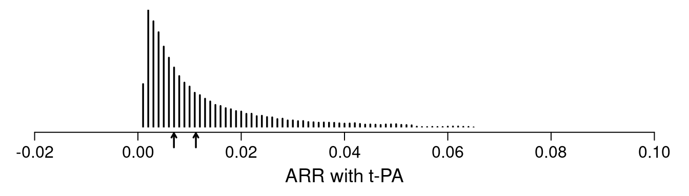
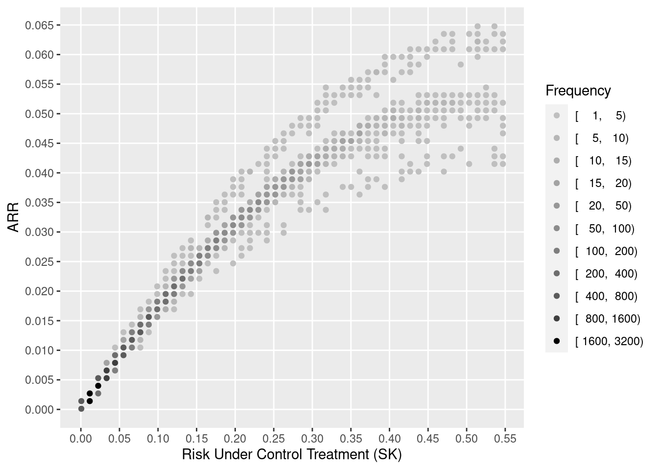
One sees the large amount of variation in ARR. Other results show large variation in risk ratios and minimal variation on ORs (and keep in mind that the optimal estimate of this OR variation is in fact zero). The relationship between baseline risk under control therapy (SK) and the estimated ARR is shown below.
Through proper conditioning and avoidance of averaging of unlikes by estimating ARR for individual patients and not averaging these estimates over patients, it is seen that standard covariate adjustment using well accepted relative treatment effect estimands is simpler, can fit data patterns better, requires only standard software, and is more insightful.
See Hoogland et al7 for a detailed article on individualized treatment effect prediction.
7 Hoogland J, IntHout J, Belias M, Rovers MM, Riley RD, Harrell FE, Moons KGM, Debray TPA, Reitsma JB (2021): A tutorial on individualized treatment effect prediction from randomized trials with a binary endpoint. Accepted, Statistics in Medicine. Preprint
8 Pearl J, Bareinboim E (2014): External validity: From do-calculus to transportability across populations. Statistical Science 29:579-595.
Others have claimed that our argument in favor of transportability of conditional estimands for treatment effects is incorrect, and that marginal estimands should form the basis for transportability of findings to other patient populations, as advocated by Pearl and Bareinboim8. The marginal estimand is not appropriate in our context for the following reasons:
- Pearl and Bareinboim developed their approach to apply to complex situations where a covariate may be related to the amount of treatment received. We are dealing only with exogeneous pre-existing patient-level covariates here.
- The transport equation 3.4 of Pearl and Bareinboim requires the use of the covariate distribution in the target population. This distribution is not usually available when a clinical trial finding is published or is evaluated by regulators.
- It is easier to transport an efficacy estimate to an individual patient (at least under the no-interaction assumption or if interactions are correctly modeled in the fully conditional model). The one patient is the target and one only needs to know her/his covariate value, not the distribution of an entire target population.
- We are ultimately interested in individual patient decision making, not group decision making.
Lack of Comparisons
Benkeser et al showed large efficiency gains of their approach over ignoring covariates. But the authors did not compare the power for their approach vs. standard covariate adjustment. This leaves readers wondering whether the new method is worth the trouble or is in fact less efficient than the standard.
New Odds Ratio Estimator
With the aim of dealing with non-proportional odds, the authors developed a weighted log odds ratio estimator. But the standard maximum likelihood estimator already solves this problem. As detailed here and here, the Wilcoxon-Mann-Whitney concordance probability \(c\), i.e., the probability that a randomly chosen patient on treatment B has a higher level response \(Y\) than a randomly chosen patient on treatment A, also called the probability index, is a simple function of the maximum likelihood estimate of the treatment regression coefficient whether or not proportional odds holds. The conversion equation is \(c = \frac{\mathrm{OR}^{0.66}}{1 + \mathrm{OR}^{0.66}}\) where OR = \(\exp(\hat{\beta})\). This formula is accurate to an average absolute error for computing \(c\) from \(\hat{\beta}\) of 0.002.
The equivalence of the OR and the Wilcoxon-Mann-Whitney estimand also makes the authors’ estimand 2 in Section 3.2 somewhat moot.
We note that overlap measures are not without problems9.
9 Senn SJ (2011): U is for unease: Reasons to mistrust overlap measures in clinical trials. Statistics in Biopharmaceutical Research 3:302-309.
Lack of a Likelihood
COVID-19 therapeutic research is an area where Bayesian methods are being used with increasing frequency. Frequentist methods that use a full likelihood approach provide an excellent bridge to development of or comparison with Bayesian analogs that use the same likelihood and only need to add a prior. The authors’ methods are not likelihood based, so they do not provide a bridge to Bayes. The proposed methods do not provide exact inference for small \(n\) as does Bayes, has no way of incorporating skepticism or external information about treatment effects, and has no way to quantify evidence that is as actionable as posterior probabilities of (1) any efficacy and (2) clinically meaningful efficacy.
The authors briefly discuss missing ordinal outcomes. Instead of this being an issue of missingness, in many situations an ordinal outcome is interval censored. This is the case, for example, when a range of ordinal values is not ascertained on a given day. To deal with interval censoring, a full likelihood approach is helpful, and the authors’ approach may not be extendible to deal with general censoring.
The lack of a likelihood also prevents the authors’ approach from dealing with variation across sites in a multi-site clinical trial through the use of random effects models, and extensions to longitudinal outcomes are not provided. The flexibility of a Bayesian longitudinal proportional odds model that allows for general censoring and departures from the proportional odds assumption is described here.
Technical Issues
The authors stated “By incorporating baseline variable information, covariate adjusted estimators often enjoy smaller variance …”. This must be clarified to apply to ARR estimates, but not in general. In logistic and Cox models, for example, covariate adjustment increases treatment effect variance on the log ratio scale (see this and this for a literature review, and also the important paper by Robinson and Jewell10). Despite this increase, traditional covariate adjustment still results in increased Bayesian or frequentist power because the model being more correct (i.e., some of the previously unexplained outcome heterogeneity is now explained) moves the treatment effect estimate farther from zero. The regression coefficient increases in absolute value faster than the standard error increases, hence the power gain. For logistic and Cox models, variance reduction occurs only on probability-scale estimands.
10 Robinson, LD, Jewell NP (1991): Some surprising results about covariate adjustment in logistic regression models. International Statistical Review 58:227-240.
In their Section 6 the authors recommended that when a utility function can be agreed upon, one should consider the difference in mean utilities between treatment arms when the outcome is ordinal. Even though the difference in mean utilities can be a highly appropriate measure of treatment effectiveness, it is important to note that the patient-specific utilities are still discrete and are likely to have a very strange, even bimodal, distribution. Hence utilities may be best modeled with a semiparametric model such as the proportional odds model.
The authors credited the proportional odds model to McCullagh11 but this model was developed by Walker and Duncan12 and other work even predates this.
11 McCullagh, P (1980): Regression models for ordinal data. Journal of the Royal Statistical Society Series B 42:109-142.
12 Walker, SH, Duncan, DB (1967): Estimation of the probability of an event as a function of several independent variables. Biometrika 54:167-178.
The authors discuss asymptotic accuracy of their method, which is of interest to statisticians but not practitioners who need to know the accuracy of the method in their (usually too small) sample.
The authors did not seem to have rigorously evaluated the accuracy of bootstrap confidence intervals. We have an example where none of the standard bootstraps provides sufficient accuracy for a confidence interval for a standard logistic model odds ratio. Non-coverage probabilities are not close to 0.025 in either tail when attempting to compute a 0.95 interval. It is important to evaluate the left and right non-coverage probabilities, as the confidence interval can be right on the average but wrong for both tails.
The use of categorization for continuous predictors (e.g., the treatment of age just before section 4.1.3) does not represent best statistical practice.
To be very picky, the authors’ (and so many other authors) use of the term “type I error” does not refer to the probability of an error but rather to the probability of making an assertion.
The paper advises readers to consider using variable selection algorithms. Stepwise variable selection brings a host of problems, typically ruins standard error estimates (Greenland13), and is not consistent with full pre-specification.
13 Greenland, S (2000): When should epidemiologic regressions use random coefficients? Biometrics 56:915-921.
The idea to use information monitoring in forming stopping rules needs to be checked for consistency with optimum decision making, and it may be difficult to specify the information threshold.
Related to missing covariates, the recommendation to use single imputation and its implication to not use \(Y\) in the imputation process has been well studied and found to be lacking, especially with regard to getting standard errors correct.
In the authors’ Supporting Information, the intuition for how covariate adjustment can lead to precision gains begins with a discussion of covariate imbalance. With the linear model, a random marginal conditional imbalance term is identified thus becoming a conditional bias, which is then removed, adjusting the estimate if necessary and reducing the variance. It is the possibility that the estimate may have to be adjusted that makes the variance for the conditional and the marginal estimates ‘correct’ given the model14. Covariate adjustment produces conditionally and unconditionally unbiased estimates. But imbalance is not the primary reason for doing covariate adjustment in randomized trials. Covariate adjustment is more about accounting for easily explainable outcome heterogeneity15 16. At any rate, apparent covariate imbalances may be offset by counterbalancing covariates one did not bother to analyze.
14 Senn SJ (2019): The well-adjusted statistician: Analysis of covariance explained. https://www.appliedclinicaltrialsonline.com/view/well-adjusted-statistician-analysis-covariance-explained . A valid standard error reflects how the estimate will vary over all randomisations. The adjustment that occurs as a result of fitting a covariate can be represented as \((Y_t - Y_c) - \beta(X_t - X_c)\). Here \(Y\) and \(X\) are means of the outcome and the covariate respectively and \(t\) stands for treatment and \(c\) stands for control. For simplicity assume the uncorrected differences at outcome and baseline have been standardised to have a variance of one. Other things being equal there cannot be a reduction in the residual variance by fitting the covariate unless \(\beta\) is large which in turn implies that \(X_t - X_c\) and \(Y_t - Y_c\) must vary together. If you don’t adjust you are allowing for the fact that in the absence of any treatment effect \(Y_t - Y_c\) might differ from 0 due to the fact that \(X_t - X_c\) differ randomly from 0 and this will affect the outcome. By adjusting you cash in the bonus by reducing the variance of the estimate. But this can only happen because adjustment is possible.
15 Lane PW, Nelder JA (1982): Analysis of covariance and standardization as instances of prediction. Biometrics 38: 613-621.
16 Senn SJ (2013): Seven myths of randomization in clinical trials. Statistics in Medicine 32:1439-1450.
Methods that develop models from only one treatment arm are prone to overfitting, which entails fitting idiosyncratic associations in that arm in such a way that when the outcome comparison is made with the other arm can result in bias in non-huge samples.
Omission of simulated samples with empty cells may slightly bias simulation results and is not necessary in ordinary proportional odds modeling.
Contrasted with the group sequential design outlined by the authors, a continuously sequential Bayesian design using a traditional proportional odds model for covariate adjustment is likely to provide more understandable evidence and result in earlier stopping for efficacy, harm, or futility.
Discussion
To add your comments, discussions, and questions go to datamethods.org here. See the end of this post for a discussion archive.
Grant Support
This work was supported by CONNECTS and by CTSA award No. UL1 TR002243 from the National Center for Advancing Translational Sciences. Its contents are solely the responsibility of the authors and do not necessarily represent official views of the National Center for Advancing Translational Sciences or the National Institutes of Health. CONNECTS is supported by NIH NHLBI 1OT2HL156812-01, ACTIV Integration of Host-targeting Therapies for COVID-19 Administrative Coordinating Center from the National Heart, Lung. and Blood Institute (NHLBI).
Discussion Archive (2021)
Lars v: Thank you for this very interesting read that leads to much thoughtful discussion. Here is some food-for-thought. Suppose was observe (X,A,Y) where X are baseline variables, A is a binary treatment, and Y is a continuous outcome. Let us assume that E[Y|A=a,X=x] = cA + dX is a linear model so that we can identify conditional effects by parameters that one can estimate at the rate square-root n (which is a big assumption). Consider, the marginal ATE effect parameter E_XE[Y|A=1,X] - E_XE[Y|A=0,X] . Under the linear model assumption, we actually have E_XE[Y|A=1,X] - E_XE[Y|A=0,X] = E_X[E[Y|A=1,X] - E[Y|A=0,X] ] = E_X[c1 + dX -c0 - dX ] = E_X[c] = c. Thus, the marginal ATE equals the conditional treatment effect parameter! This is no coincidence. Most, if not all, conditional treatment effect parameters based on parametric assumptions correspond with some nonparametric marginal treatment effect parameter (e.g. marginalized hazard ratios, odds ratios, etc). The strong parametric assumptions allow one to turn marginal effects into conditional effects. Note that simply including an interaction between A and X already makes the identification of a conditional effect parameter much more challenging. The benefit of estimating the marginal effect E_XE[Y|A=1,X] - E_XE[Y|A=0,X] instead is that our inference is non-parametrically correct even when the conditional mean is not linear. Nonetheless, there is substantial work on estimating and obtaining inference for conditional treatment effects nonparametrically (e.g. CATE). Note that this is a fairly difficult problem, as conditional treatment effect parameters are usually not square-root(n) estimable in the nonparametric setting.
As a note, this certainly motivates looking for marginal effect parameters that identify conditional effect parameters under stricter assumptions. If one is willing to believe that the assumptions are true, one can always interpret it as a conditional effect. Also, pairing estimates and inference of conditional effects based on parametric models with those of marginal effects from nonparametric models is a good way to obtain robust results that cover all bases. If the marginal effect and conditional effect are substantially different (assuming they identify the same parameter under stricter assumptions), then this might lead one to conclude that the parametric model assumptions are violated.
Frank Harrell: It’s easier to manage discussions on datamethods.org where there is a link above to a topic already started for this area. On a quick read of your interesting comments I get the idea that that thinking is restricted to linear models. If so, the scope may be too narrow.