When Equal Survival Proves Nothing

When some patients die before a response variable can be measured, comparing treatment groups on that response among survivors can be badly misleading even in a randomized trial. A popular repair assumes that treatment changes no patient’s survival, and offers equal survival in the two treatment groups as a check on that assumption. Using a simulated trial in which the truth is known exactly, this article shows that the check can pass perfectly while the survivor comparison reports a convincing treatment effect that does not exist; that no assumption about the unobservable can rescue the approach; and that what the comparison actually requires is a different and more checkable condition. A longitudinal ordinal analysis that keeps every patient asks a clinically meaningful question the data can answer and, by modeling transitions to death separately from changes in weight, recovers the true effects and shows how the assumption should have been checked. Such an analysis of everyone randomized is still causal by design. The broader lesson is that formal machinery gives false comfort when it rests on assumptions that cannot be verified, or when it quietly changes the question being asked.

Author

Affiliation

Frank Harrell

Department of Biostatistics
Vanderbilt University School of Medicine

How to cite this article

Harrell FE (2026). When Equal Survival Proves Nothing. Statistical Thinking. https://doi.org/10.59350/s8dwr-xs111

require(rms)
require(data.table)
require(tinyplot)
tinytheme('dynamic')
options(prType = 'html')

rnd  <- function(x) round(x, 3)
int  <- function(x) format(round(x), big.mark = ',')   # whole numbers in text;
                                                      # character, so knitr won't use 10^k
pct  <- function(x) round(100 * x, 1)                    # proportion -> percent
pexp <- function(p) paste0('$', latexSN(signif(p, 2)), '$')
r2   <- function(fit) {                                   # last-listed R^2
  s <- fit$stats
  unname(s[max(grep('^R2', names(s)))])
}
res  <- list()                                            # quantities quoted in the text

Executive Summary

• The problem. When death occurs before a non-mortality outcome \(Y\) is assessed, \(Y\) is undefined, not missing. Comparing \(Y\) among survivors loses the protection of randomization, because survival happens after randomization and may itself depend on treatment. → The Question
• A popular repair. Estimate the effect among patients who would survive on either treatment, assume treatment changes no one’s survival, and check that survival is equal in the two arms. → A Proposed Repair
• The check can pass while the answer is badly wrong. In a simulated trial where treatment has no effect on weight and overall survival is equal by design, the survivor comparison reports a highly significant effect on weight that does not exist. → A Simulated Trial · → The Survivor Comparison Gets the Wrong Answer
• No assumption about the unseeable rescues it. The assumption concerns pairs of outcomes no patient can reveal. The check can only refute it, and is blind to treatment saving some patients while killing others. Weaker substitutes are equally unverifiable, and the target group cannot be identified by any clinician. → No Assumption About the Unseeable · → What the Comparison Actually Requires
• A better question. Count every randomized patient: each week a patient is alive at some value of \(Y\), or dead, an absorbing state. This leads to intention-to-treat estimates such as \(P(Y < y \text{ and alive})\) rather than \(P(Y < y \mid \text{alive})\). → Data-Informed Answer
• Separate transition models find the truth. Modeling death separately from changes in \(Y\) among the living finds no effect on weight and opposite effects on death in different kinds of patients. It rejects the assumption decisively where the overall check could not. → What the Transition Model Finds
• Its assumptions can be checked. Every assumption of this approach concerns observed data and can be tested and relaxed. → Assumptions That Can Be Checked
• The lesson. Formal machinery gives false comfort when it rests on assumptions no data can verify, or when it quietly changes the question. An analysis of everyone randomized is causal by design. → What Formalism Can and Cannot Do

Discussion Board

Background

Proponents of causal formalism claim it is indispensable for justifying claims of causal effects of interventions, even in carefully controlled randomized experiments. As argued in Harrell (2026a) and addressed with purely statistical models in Harrell (2026b), straight-up randomized trials are causal by design and do not require causal formalism. Formalists claim that even if this is the case, “broken” randomized clinical trials (RCTs), such as RCTs with post-randomization exclusions, require causal formalism to justify attribution of treatment differences to treatment. They go on to say that even the simplest unbroken RCT profits from causal formalism because the formalism provides a bridge to dealing with broken RCTs. The problem is that a widely offered formal repair for an important class of broken RCTs rests on an assumption about outcomes that can never be observed, accompanied by a check that is blind to the way the assumption is most likely to fail. This article shows that a better analysis, based entirely on what was observed, needs neither.

The Question

Consider a specific RCT in which the outcome is truncated by death, so that an analysis restricted to survivors loses the protection provided by randomization. In an example offered by Iván Díaz on X on 2026-09-10 and summarized and discussed here, suppose a trial compares two antidepressants. Weight gain is a well-known side effect of many such drugs, so a natural secondary question is how much the newer drug changes weight compared with the older one. I suppose that each patient’s weight is intended to be measured every week for the duration of the trial, and some patients die during follow-up.

For a patient who dies, weight after death is not missing in the usual sense. It does not exist. So what does “the effect of treatment on weight” mean when not everyone is alive to be weighed? The simplest analysis compares average weight at the end of the trial between the treatment groups, among the patients still alive. This is tempting and often wrong. Randomization makes the two treatment groups comparable at the start of the trial. It does not make comparable a subset of patients selected by something that happened after randomization, and survival is exactly such a thing. If treatment affects who survives, the survivors in one group can be a different kind of patient from the survivors in the other, and a difference in their weights may say nothing at all about what treatment does to weight.

Regulatory guidance unsatisfyingly calls death an intercurrent event : something that happens after treatment starts and affects whether or how the outcome can be measured. See the ICH E9(R1) addendum and the primer by Kahan et al. (2024).

A Proposed Repair

One way out is to change what is being estimated. Instead of the effect of treatment on everyone randomized, estimate the effect among patients who would have survived whichever treatment they were given. This repair comes from a way of thinking that imagines, for every patient, two outcomes: what would happen on one treatment and what would happen on the other. Only one of the two can ever be seen. If treatment changes no patient’s survival—if every patient who survives on one treatment would also survive on the other, and every patient who dies on one would also die on the other—then the survivors in the two groups are the same kind of patient, randomization still protects the comparison, and the simple survivor comparison estimates that effect.

This is the potential outcomes framework of causal inference (Rubin 1974). \(S(A)\) is a patient’s potential survival outcome: whether the patient would survive if given treatment \(A\) (\(A\) = 0 for control, 1 for active). The assumption is \(S(1) = S(0)\) for every patient. Patients are grouped into principal strata by their pair \((S(0), S(1))\), and the target is the treatment effect within the stratum of “always survivors” (Frangakis and Rubin 2002; Rubin 2006), often called the survivor average causal effect. Without the assumption, that effect is not identified from the data; bounds and estimates under other unverifiable assumptions are developed in Zhang and Rubin (2003), Hayden et al. (2005), and Ding et al. (2011). The role of this principal stratum strategy in drug development is reviewed by Bornkamp et al. (2021).

The assumption is strong, and its defenders offer a check. Díaz stated it as “treatment changes no individual’s survival” and pointed out that it “implies P(S=1|A=1)=P(S=1|A=0), so the assumption is falsifiable.” In words: if treatment changes no one’s survival, the proportion surviving must be the same in both treatment groups. That is correct. Published guidance on handling death in trials goes a step further, describing the assumption as “testable, since it implies comparable survival across arms” (Pham et al. 2025).

The difference between those two statements matters. Falsifiable means that a failed check refutes the assumption. Testable suggests something more—that a passed check supports it. Unequal survival would indeed refute the assumption, but equal survival need not support it, because treatment could save some patients and kill an equal number of others.

If A implies B, observing B does not establish A. Reasoning otherwise is the logical error known as affirming the consequent.

So how much comfort should a passed check give? The way to find out is to study a trial in which the truth is known.

A Simulated Trial Where the Truth Is Known

m      <- 26        # weeks of scheduled follow-up
npg    <- 6000      # patients per treatment group
pfrail <- 0.5       # probability that a patient is frail
wlev   <- c(frail = 60, robust = 80)   # means of true weight levels (kg)
sdlev  <- 5         # between-patient SD of true weight level (kg)
sdmeas <- 3         # SD of week-to-week variation of a patient's weight
                    # around their true level (kg)
wtdead <- 1000      # weight value used to record death; exceeds every real
                    # weight, so death is automatically the worst outcome

##  Probability of surviving to week m, by kind of patient and treatment.
##  Defined once here so that the data generator, the tables, and the
##  reference lines in the figures can never disagree.
psurv <- matrix(c(0.80, 0.90,          # frail:  treatment helps
                  0.95, 0.85),         # robust: treatment harms
                nrow = 2, byrow = TRUE,
                dimnames = list(c('frail', 'robust'), c('control', 'active')))
overall <- as.vector(c(pfrail, 1 - pfrail) %*% psurv)

The simulated trial randomizes 6,000 patients to each of two treatments and weighs every patient once a week for 26 weeks. The data are generated so that two things are true by construction: treatment has no effect on any patient’s weight, and the overall proportion of patients surviving is identical in the two treatment groups.

There are two kinds of patients, and the investigator cannot tell them apart. Frail patients tend to be lighter, with true weight levels centered at 60 kg. Robust patients tend to be heavier, centered at 80 kg. A patient is frail with probability 0.5. Treatment helps frail patients survive and harms robust ones. The chance of surviving to week 26 is:

tab <- rbind(psurv, overall)
dimnames(tab) <- list(c('Frail (lighter)', 'Robust (heavier)', 'All patients'),
                      c('Control', 'Active'))
knitr::kable(tab, digits = 3)

Table 1: Probability of surviving to the end of follow-up, by kind of patient and treatment. Frailty is never observed by the investigator.

	Control	Active
Frail (lighter)	0.800	0.900
Robust (heavier)	0.950	0.850
All patients	0.875	0.875

The gains among frail patients exactly offset the losses among robust ones, so the overall chance of survival is 0.875 under control and 0.875 under the active treatment.

Each patient’s true weight level varies around the mean for their kind, with a standard deviation of 5 kg, and each week’s weight varies independently around the patient’s true level with a standard deviation of 3 kg. This within-patient variation stands for everything that makes one week’s weight differ from the next for the same patient: genuine fluctuation from meals, fluid balance and activity, as well as the error of the scale. The simulation, and the analysis, do not need to separate the two. Weight is recorded at baseline (week 0) and every week while the patient is alive. The record simply ends at death. Treatment appears nowhere in the weight process. Figure 1 summarizes the structure.

Figure 1: How the simulated data are generated, and why a comparison of survivors fails. Frailty (dashed border) is never observed; it determines both how heavy a patient is and how likely they are to die. Treatment affects only the chance of dying, helping frail patients and harming robust ones, and has no effect on anyone’s weight. Death ends a patient’s weight record. Restricting attention to survivors opens the path treatment → death ← frailty → weight: because survival depends on both treatment and frailty, treated and control survivors differ in frailty, and therefore in weight. In DAG language, survival is a collider.

Survival is governed by a constant weekly risk of death, set by the patient type and treatment to reproduce the probabilities above. One more device makes the simulation useful for our purpose. Each patient carries a single random number that determines when they would die under either treatment, and the treatment they were actually randomized to decides which of the two outcomes we get to see. These are exactly the two potential outcomes the repair is built on. No real trial can see both, but a simulation can, and that lets us count exactly how many patients treatment saved or killed instead of arguing about it.

Sharing one random number between the two treatments links the patient’s two potential survival outcomes so that they agree as often as possible (a comonotonic coupling). It is therefore the arrangement most favorable to the assumption that treatment changes no one’s survival.

Figure 2 lays out every step of the data-generating model for one patient, and the function below implements it.

Figure 2: The data-generating model for one patient. Dashed boxes are never seen by the investigator. Treatment enters only through the probability of surviving; no path leads from treatment to the weight process. A single random number V determines when the patient would die under either treatment, which links the two potential survival outcomes (dotted box) as closely as possible; they are used only to count the patients whom treatment saved or killed, never in any analysis. Parameter values are set in the parameters code chunk.

##  Generate the record of ONE patient.
##    tx : 0 = control, 1 = active treatment
##    m  : weeks of scheduled follow-up
##
##  Frailty U (1 = frail, 0 = robust) is never seen by the investigator.
##  It sets the true weight level and the risk of dying, and is the only
##  link between weight and death.  Treatment enters ONLY the survival
##  probability, never the weight process.
##
##  Records returned, one per scheduled visit:
##    weeks 0, 1, ..., tlast   real weights; tlast is the last scheduled
##                             week strictly before death (capped at m)
##    one further record       only if death occurs during follow-up: week
##                             tlast + 1 with wt = wtdead
##  A patient alive at week m has exactly m + 1 records.  Nothing is missing.
##
##  U, S0 and S1 are the unobservable truth, returned only so the article
##  can report what the design did.  No analysis below ever uses them.

gen1 <- function(tx, m) {
  U      <- rbinom(1, 1, pfrail)                    # 1 = frail, 0 = robust
  level  <- wlev[2L - U] + rnorm(1, 0, sdlev)       # true weight level, kg
  p      <- psurv[2L - U, ]                         # c(control, active)
  ##  One random number per patient, shared by both treatments.  Surviving
  ##  to week m under treatment a is exactly V < p[a].
  V      <- runif(1)
  tdeath <- -log(V) / (-log(p[tx + 1L]) / m)        # constant weekly hazard
  S0     <- V < p['control']                        # survives under control?
  S1     <- V < p['active' ]                        # survives under active?
  ##  as.integer() matters: data.table needs the same column type for every
  ##  patient, and ceiling() returns a double
  tlast  <- as.integer(min(m, ceiling(tdeath) - 1))
  week   <- 0L : tlast
  wt     <- level + rnorm(length(week), 0, sdmeas)  # no treatment term
  if(tdeath <= m) {                                 # death during follow-up
    week <- c(week, tlast + 1L)
    wt   <- c(wt,   wtdead)
  }
  data.table(week = week, wt = wt, U = U, S0 = S0, S1 = S1)
}

The generator is run once for every patient. The grid crosses a patient number with treatment, giving 6,000 patients in each group.

set.seed(23)
grid <- setDT(expand.grid(i = 1 : npg, m = m, tx = 0 : 1))
grid[, id := .I]
dall <- grid[, gen1(tx, m), by = .(id, tx)]
dall[, dead := wt == wtdead]
dall[, wt0  := wt[week == 0], by = id]                 # baseline weight

What the Design Guarantees

b0   <- dall[week == 0, .(mean = mean(wt), sd = sd(wt)), by = tx][order(tx)]
surv <- dall[, .(alive = ! any(dead)), by = .(id, tx)]
sm   <- surv[, .(n = .N, alive = sum(alive)), by = tx][order(tx)]
tru  <- dall[week == 0, .(tx, U, S0, S1)]

res <- c(res, list(
  b0mean = b0$mean,
  b0sd   = b0$sd,
  b0p    = t.test(wt ~ tx, data = dall[week == 0])$p.value,
  b0ks   = suppressWarnings(ks.test(dall[week == 0 & tx == 0, wt],
                                    dall[week == 0 & tx == 1, wt])$p.value),
  surv   = sm$alive / sm$n,
  survp  = prop.test(sm$alive, sm$n)$p.value,
  disc   = tru[, mean(S0 != S1)],
  saved  = tru[, mean(! S0 &   S1)],
  killed = tru[, mean(  S0 & ! S1)]))

The simulated trial behaves exactly as designed. Mean baseline weight is 70.1 kg (SD 11.435) in the control group and 70.099 kg (SD 11.558) in the active group. Because both groups are drawn from the same distribution, any difference is due to chance alone (P = \(1\) for the means, \(0.77\) for the whole distributions). Overall survival to week 26 is 0.875 under control and 0.874 under the active treatment, and a test of equal survival gives P = \(0.98\).

The distributions are compared with the Kolmogorov–Smirnov test, survival proportions with the \(\chi^2\) test.

The check passes. Yet treatment changed whether 9.8% of patients survived: it saved 4.6% of patients who would have died on control, and killed 5.2% who would have lived.

The Survivor Comparison Gets the Wrong Answer

wm <- dall[week == m & ! dead]
tt <- t.test(wt ~ tx, data = wm)        # estimates control - active
res <- c(res, list(
  survcon    = wm[tx == 1, mean(wt)] - wm[tx == 0, mean(wt)],
  survcon_ci = sort(- tt$conf.int),
  survcon_p  = tt$p.value,
  frail0     = tru[, mean(U), by = tx][order(tx), V1],   # at randomization
  frailm     = dall[week == m & ! dead, mean(U), by = tx][order(tx), V1]))

Now do what an analyst might do: compare week-26 weights among patients still alive. Survivors on the active treatment weigh -1.122 kg relative to survivors on control (0.95 confidence interval -1.563 to -0.681, P = \(6.1\times 10^{-7}\)). The report would say the new drug lowers weight, with overwhelming statistical evidence. In truth, it changes no patient’s weight at all.

The reason is the one Figure 1 predicts. At randomization the proportion of frail patients is 0.495 in the control group and 0.494 in the active group. Among patients still alive at week 26 it is 0.455 and 0.512. Treatment kept more of the light patients alive and fewer of the heavy ones, so its survivors are lighter. Randomization balanced the groups; mortality unbalanced the survivors.

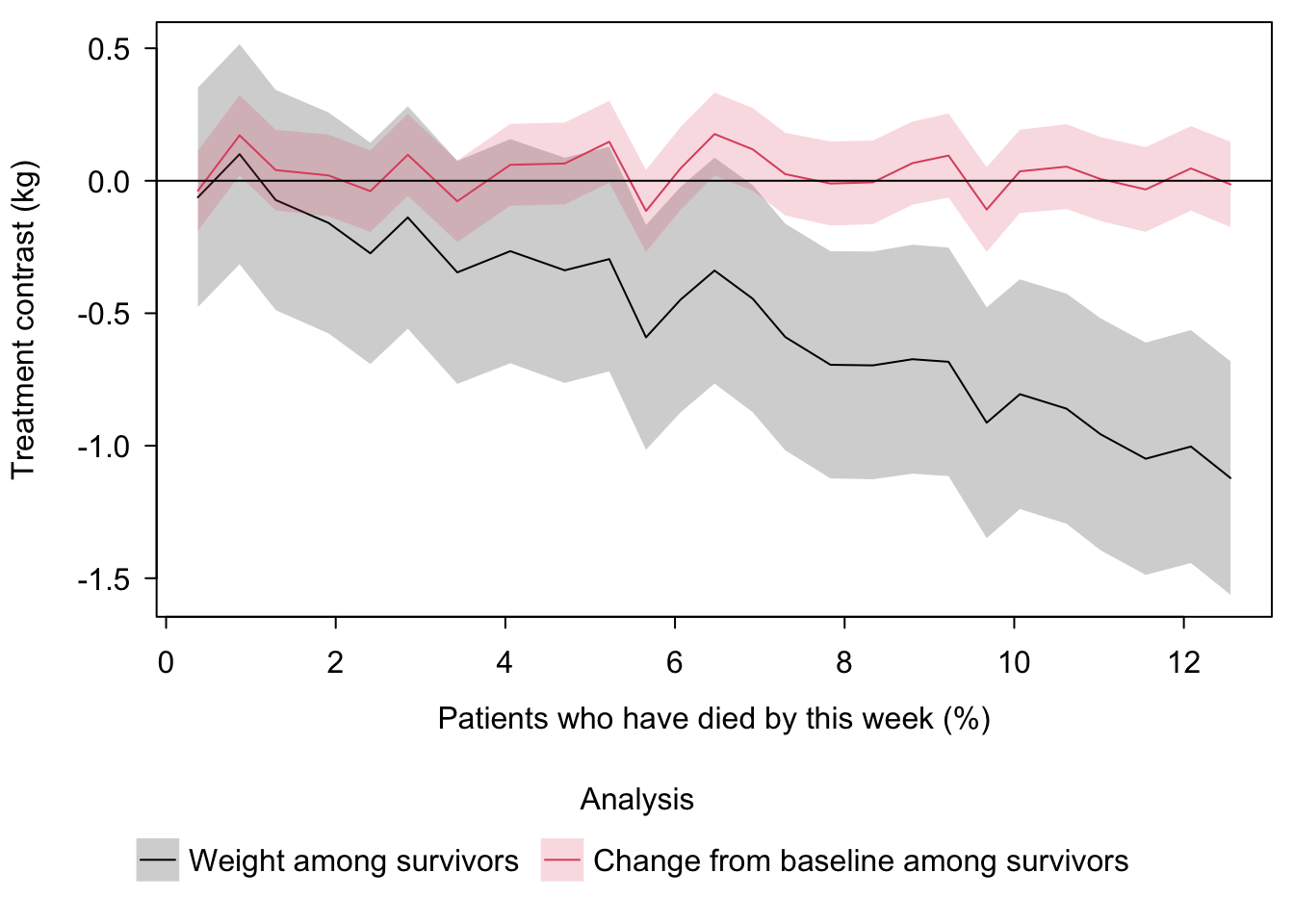
A signature of this kind of artifact is that it is created by deaths. Before anyone has died there is nothing to unbalance, so the apparent effect must start at zero and grow as deaths accumulate. A real effect of treatment on weight is under no such constraint. A second clue comes from looking at each patient’s change from their own baseline weight instead of their weight level. Selection by death acts on how heavy a patient is, and subtracting each patient’s baseline weight removes that.

Change from baseline is used here as a diagnostic, not as a recommended analysis. Its usual drawbacks are discussed here.

npat <- uniqueN(dall$id)

##  A patient alive at week t has exactly one record at week t; a patient
##  who died earlier has none.  So counting records gives both the number
##  at risk and cumulative mortality.
tc <- dall[dead == FALSE & week >= 1, {
  y1 <- wt[tx == 1]
  y0 <- wt[tx == 0]
  c1 <- (wt - wt0)[tx == 1]
  c0 <- (wt - wt0)[tx == 0]
  .(nalive    = .N,
    level     = mean(y1) - mean(y0),
    level_se  = sqrt(var(y1) / length(y1) + var(y0) / length(y0)),
    change    = mean(c1) - mean(c0),
    change_se = sqrt(var(c1) / length(c1) + var(c0) / length(c0)))
}, by = week][order(week)]
tc[, pct_dead := 100 * (1 - nalive / npat)]

L <- melt(tc,
          id.vars       = .q(week, pct_dead),
          measure.vars  = list(.q(level, change), .q(level_se, change_se)),
          value.name    = .q(est, se),
          variable.name = 'analysis')
L[, analysis := factor(analysis, 1 : 2,
                       c('Weight among survivors',
                         'Change from baseline among survivors'))]
L[, `:=`(lo = est - 1.96 * se, hi = est + 1.96 * se)]

res <- c(res, list(
  r_level   = cor(tc$level, tc$pct_dead),
  level_m   = tc[week == m, level],
  change_m  = tc[week == m, change],
  change_se = tc[week == m, change_se],
  pctdead_m = tc[week == m, pct_dead]))

cap_artifact <- paste0(
  'Treatment contrasts among patients still alive, plotted against the ',
  'percentage who have died by that week, with 0.95 confidence bands. ',
  "Treatment changes no patient's weight, yet the contrast in weight level ",
  'tracks cumulative mortality almost exactly (r = ', rnd(res$r_level),
  '), reaching ', rnd(res$level_m), ' kg once ', round(res$pctdead_m, 1),
  '% have died. The contrast in change from baseline, which cancels the ',
  'weight level that mortality selects on, stays near zero throughout.')

plt(est ~ pct_dead | analysis, data = L, ymin = lo, ymax = hi,
    type = type_ribbon(),
    xlab = 'Patients who have died by this week (%)',
    ylab = 'Treatment contrast (kg)',
    legend = list('bottom!', title='Analysis'))
abline(h = 0, lty = 1)

Figure 3: Treatment contrasts among patients still alive, plotted against the percentage who have died by that week, with 0.95 confidence bands. Treatment changes no patient’s weight, yet the contrast in weight level tracks cumulative mortality almost exactly (r = -0.97), reaching -1.122 kg once 12.5% have died. The contrast in change from baseline, which cancels the weight level that mortality selects on, stays near zero throughout.

Figure 3 shows both. The contrast in weight among survivors grows in almost perfect proportion to cumulative mortality, while the contrast in change from baseline stays close to zero, ending at -0.014 kg with a standard error of 0.082.

The change contrast wanders a little because each patient’s single baseline weight, with its own week-to-week variation, is shared by all of that patient’s later weeks. Its wandering is consistent with chance.

NoteWhy not simply analyze change from baseline?

Figure 3 invites an obvious question: if change from baseline removes the artifact, why not start there? There are four reasons, and the first explains why it works here at all.

It works here by construction. In the simulation, frailty shifts only a patient’s level of weight. Each weekly weight is that fixed level plus independent week-to-week variation. Change from baseline is (level + this week’s variation) − (level + baseline variation), so the level cancels exactly. Frailty is the only thing survival selects on, so nothing left in the change score can differ between the survivor groups. The flat right-hand panel of Figure 3 is a property of this data-generating model, not a property of change scores.

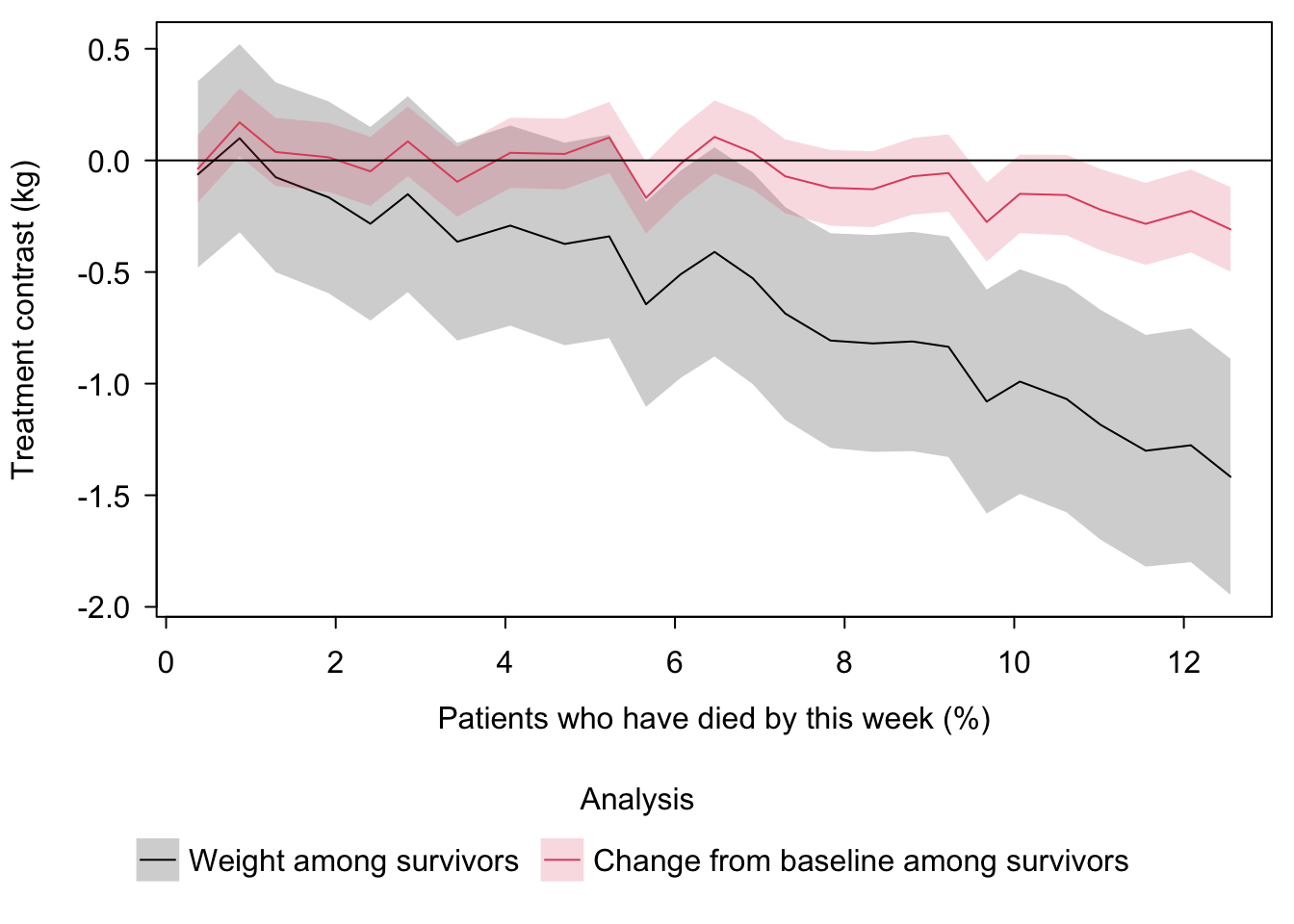
In real trials it usually will not work. Death selects on whatever distinguishes patients who are about to die, and that typically includes their trajectory, not just their level: weight often falls in the months before death. If treatment keeps more of the declining patients alive, its survivors show more weight loss, and subtracting baseline does nothing about selection on trajectory. To see this, the code below takes the simulated trial exactly as it is—same patients, same deaths—and makes one change: frail patients lose weight steadily while they are alive, at the rate wslope set in the code. Treatment still has no effect on anyone’s weight.

##  Same patients, same deaths; frail patients' real weights now decline
##  by |wslope| kg per week while they are alive.  Treatment still has no
##  effect on weight.  Baseline (week 0) weights are unchanged.
wslope <- -0.2
dv <- copy(dall)
dv[dead == FALSE & U == 1, wt := wt + wslope * week]

tcv <- dv[dead == FALSE & week >= 1, {
  y1 <- wt[tx == 1]
  y0 <- wt[tx == 0]
  c1 <- (wt - wt0)[tx == 1]
  c0 <- (wt - wt0)[tx == 0]
  .(nalive    = .N,
    level     = mean(y1) - mean(y0),
    level_se  = sqrt(var(y1) / length(y1) + var(y0) / length(y0)),
    change    = mean(c1) - mean(c0),
    change_se = sqrt(var(c1) / length(c1) + var(c0) / length(c0)))
}, by = week][order(week)]
tcv[, pct_dead := 100 * (1 - nalive / npat)]

Lv <- melt(tcv,
           id.vars       = .q(week, pct_dead),
           measure.vars  = list(.q(level, change), .q(level_se, change_se)),
           value.name    = .q(est, se),
           variable.name = 'analysis')
Lv[, analysis := factor(analysis, 1 : 2,
                        c('Weight among survivors',
                          'Change from baseline among survivors'))]
Lv[, `:=`(lo = est - 1.96 * se, hi = est + 1.96 * se)]

res <- c(res, list(
  v_change_m  = tcv[week == m, change],
  v_change_se = tcv[week == m, change_se],
  v_r_change  = cor(tcv$change, tcv$pct_dead)))

cap_slope <- paste0(
  'The same treatment contrasts as in @fig-artifact, for the same simulated ',
  'patients and deaths, except that frail patients lose ', abs(wslope),
  ' kg per week while alive. Treatment still changes no patient\'s weight, ',
  'but now the contrast in change from baseline also tracks cumulative ',
  'mortality (r = ', rnd(res$v_r_change), '), reaching ',
  rnd(res$v_change_m), ' kg (standard error ', rnd(res$v_change_se),
  ') at week ', m, '.')

plt(est ~ pct_dead | analysis, data = Lv, ymin = lo, ymax = hi,
    type = type_ribbon(),
    xlab = 'Patients who have died by this week (%)',
    ylab = 'Treatment contrast (kg)',
    legend = list('bottom!', title = 'Analysis'))
abline(h = 0, lty = 1)

Here frail patients lose 0.2 kg per week. In Figure 4 the change-from-baseline contrast is no longer flat. It grows with cumulative mortality, reaching -0.309 kg (standard error 0.097) at week 26, for a treatment that does nothing to weight. The simulation in the main text is therefore the case most favorable to change scores, and should not be read as showing that change scores solve truncation by death. Whether a particular transition model removes selection of this kind is itself something that can be checked from the data, by the methods listed in Assumptions That Can Be Checked below.

It is still an analysis of survivors only. Even when change from baseline removes the bias, it answers a question about the patients who lived and uses nothing from the deaths. It could never find what the transition models find below: that treatment has opposite effects on death in light and heavy patients. The point of the analysis recommended here is to keep every randomized patient, and a survivor-only change-score analysis does not.

Change scores are an inefficient use of baseline even without death. Subtracting baseline forces the coefficient of baseline weight to be exactly 1. Week-to-week variation makes the true relationship between baseline and later weight weaker than that, which produces regression to the mean. Treating baseline as a covariate is more efficient and imposes no such constraint, and the transition models go further, using baseline weight and the previous week’s weight with flexible shapes. Change scores also carry each patient’s baseline variation into every later week, which is why the change contrast in Figure 3 wanders. These drawbacks are discussed here.

The legitimate role of change from baseline here is diagnostic. It reveals what survival selected on. When the level contrast tracks mortality and the change contrast stays flat, the selection is on level. When both track mortality, as in Figure 4, the selection is on trajectory as well, a warning that no simple survivor analysis is safe. The transition models are what answer the question.

Figure 4: The same treatment contrasts as in , for the same simulated patients and deaths, except that frail patients lose 0.2 kg per week while alive. Treatment still changes no patient’s weight, but now the contrast in change from baseline also tracks cumulative mortality (r = -0.764), reaching -0.309 kg (standard error 0.097) at week 26.

No Assumption About the Unseeable Can Rescue It

In a real trial no one ever sees both survival outcomes for the same patient: each patient receives one treatment, and what would have happened on the other is never observed. How a patient’s two hypothetical outcomes go together cannot be learned from any data, however many patients are studied (Dawid 2000; Senn 2004; Senn et al. 2011; Dawid and Senn 2023). One might therefore suspect that the simulation stacked the deck by choosing a convenient way for the two outcomes to go together.

It did the opposite. Within each kind of patient, the two survival probabilities in Table 1 differ, and that alone forces a minimum number of patients whose survival treatment changes, whatever is assumed about the unobservable. The table below shows how many patients have their survival changed by treatment under different ways the two outcomes could go together, all consistent with this design.

p0  <- psurv[, 'control']
p1  <- psurv[, 'active' ]
w   <- c(pfrail, 1 - pfrail)
cpl <- rbind(abs(p1 - p0),                           # outcomes agree when possible
             p1 * (1 - p0) + p0 * (1 - p1),           # independent
             abs(p1 - p0),                           # smallest possible
             p1 + p0 - 2 * pmax(0, p1 + p0 - 1))      # largest possible
cpl <- cbind(cpl, overall = as.vector(cpl %*% w))
res <- c(res, list(
  floor   = cpl[3, 'overall'],
  savemin = sum(w * pmax(0, p1 - p0)),           # fewest patients saved
  killmin = sum(w * pmax(0, p0 - p1)),           # fewest patients killed
  ceil    = cpl[4, 'overall']))
dimnames(cpl) <- list(c('As simulated (agree as often as possible)',
                        'Independent',
                        'Smallest possible',
                        'Largest possible'),
                      c('Frail', 'Robust', 'All patients'))
knitr::kable(100 * cpl, digits = 1)

Table 2: Percent of patients whose survival to week 26 would differ between the two treatments (saved plus killed), under different ways a patient’s two potential survival outcomes could be linked. Every row is consistent with the same design; the data can never say which is true.

	Frail	Robust	All patients
As simulated (agree as often as possible)	10	10.0	10.0
Independent	26	18.5	22.2
Smallest possible	10	10.0	10.0
Largest possible	30	20.0	25.0

The simulation used the arrangement that makes the two outcomes agree as often as possible, which yields the smallest possible number of patients affected. Even so, treatment changes the survival of 10% of patients, and it could be as many as 25%. The assumption fails by at least 10 percentage points no matter what one believes about quantities no experiment can reveal.

The smallest and largest possible values are the Fréchet–Hoeffding bounds. For two yes/no outcomes with probabilities \(p_0\) and \(p_1\), the proportion disagreeing must lie between \(|p_1 - p_0|\) and \(\min(p_0 + p_1, 2 - p_0 - p_1)\).

NoteWhat “percent of patients whose survival is changed by treatment” means

The quantity in Table 2 is the percentage of patients whose survival to the end of follow-up (week 26) would be different on the two treatments. In potential-outcome terms it is the proportion of patients with \(S(0) \neq S(1)\), which is the sum of two kinds of patients:

• saved: \(S(0) = 0\) and \(S(1) = 1\), dying on control but surviving on the active treatment, and
• killed: \(S(0) = 1\) and \(S(1) = 0\), surviving on control but dying on the active treatment.

The Frail and Robust columns give \(\Pr(S(0) \neq S(1) \mid U = u)\) within each kind of patient. The All patients column averages the two, weighted by the proportion of each kind (0.5 frail and 0.5 robust).

Why several rows? Data, even unlimited data, determine only the two survival probabilities within each kind of patient, \(p_{0u} = \Pr(S(0) = 1 \mid u)\) and \(p_{1u} = \Pr(S(1) = 1 \mid u)\). How often a patient’s two outcomes disagree depends also on how the two are linked within a patient, and no trial can observe that. Each row is one possible linking:

Row	\(\Pr(S(0) \neq S(1) \mid u)\)
As simulated (agree as often as possible)	\(\lvert p_{1u} - p_{0u} \rvert\)
Independent	\(p_{1u}(1 - p_{0u}) + p_{0u}(1 - p_{1u})\)
Smallest possible	\(\lvert p_{1u} - p_{0u} \rvert\)
Largest possible	\(\min(p_{0u} + p_{1u},\ 2 - p_{0u} - p_{1u})\)

The first and third rows are equal because the simulation’s shared random number produces the smallest possible disagreement. The table gives the values implied by the design; the proportion actually realized among the simulated patients, 9.8%, is quoted in What the Design Guarantees, and differs from the design value of 10% only by chance.

Two limits are worth keeping in mind. First, the quantity counts only whether a patient is alive at week 26. A patient who would die on both treatments, but in different weeks, counts as unchanged even though treatment changed when they died, so the table understates how much treatment changes survival time. Second, it is a property of the joint distribution of potential outcomes, which can never be observed. That is the point of the table: only the smallest and largest possible values follow from the observable survival probabilities, and even the smallest is far from the zero that the assumption requires.

The strongest case for the survivor approach does not rest on the assumption that treatment changes no one’s survival. Careful analysts often replace it with weaker ones that also need to be addressed. The most common is monotonicity: treatment may save some patients but kill none, or the reverse. It fails here as well, under every possible linking of the two outcomes: at least 5% of patients are saved by treatment and at least 5% are killed by it. Another approach assumes that, once measured covariates are taken into account, which stratum a patient belongs to carries no further information about the outcome (principal ignorability, Ding and Lu 2017). That is again an assumption about pairs of outcomes no one can observe together. A third approach gives up a single answer and reports the range of values consistent with the data (Zhang and Rubin 2003). That is honest, but the range is often wide, and it is still a range for the effect in a group of patients nobody can identify. Each step toward weaker assumptions buys credibility at the price of usefulness, and none of them removes the dependence on what can never be seen. For the simulated trial the smallest possible percentages of patients saved and killed are \(\sum_u \Pr(u) \max(0, p_{1u} - p_{0u})\) and \(\sum_u \Pr(u) \max(0, p_{0u} - p_{1u})\), where \(u\) indexes the kind of patient. Both are positive, so treatment both saves and kills under every linking consistent with the design.

What the Survivor Comparison Actually Requires

A deeper point is that the survivor comparison does not actually need the strong assumption that treatment changes no patient’s survival. It needs only that the survivors in the two groups be the same mix of patients, in every respect that affects weight. Because randomization makes the groups the same mix at the start, that holds if, within each kind of patient, treatment does not change the chance of surviving.

This weaker condition is about groups of patients, not about each patient’s two hypothetical outcomes, so it requires no speculation about what can never be observed. Frailty was not measured in this trial, but it could be measured in principle; the way a patient’s survival on one treatment goes with their survival on the other cannot be measured even in principle. It also makes plain what the offered check misses. The condition that matters is about survival within kinds of patients. The check looks only at survival overall. Here, within frail patients treatment raises survival from 0.8 to 0.9; within robust patients it lowers survival from 0.95 to 0.85. Overall, survival is unchanged. The gap between “within” and “overall” is exactly where effects that cancel each other exist, and is invisible to the check.

Formally, the comparison needs survival to be independent of treatment given the factors \(U\) that also affect weight: \(\Pr(S = 1 \mid A, U)\) must not depend on \(A\). This is a statement about a single world, involving no joint distribution of potential outcomes, and it is weaker than \(S(1) = S(0)\).

The assumption is also implausible exactly where it matters most. In an antidepressant trial, a possible effect of treatment on survival is not a technicality; it is the central safety question. Assuming treatment changes no one’s survival assumes away the very concern that makes the analysis difficult.

The weaker condition still cannot be checked when the relevant kinds of patients are invisible. But the data often contain partial information about them, for a reason that is not specific to this example. A survivor comparison of weight can be biased only by something that affects both survival and weight. Whatever affects weight leaves traces in the weights recorded before death. The same thing that creates the bias therefore tends to create evidence that can be used to detect and remove it. Here, weight itself reflects frailty. That suggests a different approach: instead of an analysis that throws away everyone who died and then assumes the problem away, use all the data, including the deaths.

Data-Informed Answer

When death makes the original question unanswerable, a reasonable response is to ask a clinically meaningful question that the data can answer, rather than to adopt a stronger assumption that rescues the original one. The road to a better solution begins with recognizing the trial as a longitudinal study.

Each week, every patient is in one of a set of ordered states: alive at some weight, or dead. Death is ranked worse than any weight, and among the living a heavier weight is ranked worse than a lighter one. A natural question is then: does assignment to the active treatment tend to put patients in better or worse states over time? This question is defined for every randomized patient, it matters to patients and clinicians, and the data answer it directly, with no assumption about outcomes that were never observed. Ranking death against the weights is needed only to summarize everything in a single number. The separate analyses of death and of weight in the next section need no such ranking, and they answer more specific questions: how treatment affects the chance of dying, and how it affects weight among those alive.

This treats the weekly outcome as ordinal. An ordinal analysis uses only the ordering of the states, not any numerical spacing between them, so it never has to decide how many kilograms a death is “worth.” That distinguishes it from composite outcomes that assign death a numerical value, where the choice of value changes the answer (Pham et al. 2025).

This reformulation also changes the question, and it is fair to ask how it differs from changing the question to “patients who would live either way.” The difference is that the reformulated question is still about everyone randomized, it describes something a clinician could act on, and every part of it is estimable from the data. The question about patients who would live either way concerns a group that cannot be identified before treatment—no clinician can tell whether the patient in front of them belongs to it—and its answer depends on assumptions the data cannot check. Matching the analysis to the research question when follow-up is truncated by death is discussed by Kurland et al. (2009), and the options for functional outcomes in trials with high mortality are compared by Colantuoni et al. (2018). How intercurrent events such as death change the question being asked is examined by Stensrud and Dukes (2022).

The model describes each week’s state in terms of the previous week’s state, the patient’s baseline weight, time, and treatment. Weight enters as measured, with no binning or rounding, and death is simply the worst possible value. The first model makes three choices that the analyses in the next section do not: it ranks death as worse than any weight, it assumes proportional odds across the whole spectrum of states including the boundary between life and death, and it therefore forces a single treatment effect to describe both the chance of dying and the distribution of weight. This is a MOST (Markov ordinal state transition) model, covered in an extensive tutorial (Rohde et al. (2024)) and here. The model is a first-order Markov proportional odds model: first-order Markov because each week’s state is modeled from the previous week’s state; proportional odds because treatment is assumed to shift the whole distribution of states in a specific way (parallelism of logits of cumulative distribution functions). That assumption can be relaxed with a partial proportional odds model, or avoided across the life–death boundary altogether by modeling death and weight with separate transition models, as is done in the next section. See these notes for details and this resource for ordinal models generally. Baseline weight is included as a separate term, not only as the previous state at week 1, so it can have a permanent effect: it is a second weight that varies around the same true level, and so carries further information about that level and about frailty.

##  Transitions: attach the previous week's weight to each week's record.
##  The inner self-join also drops week 0, which has no predecessor.  No
##  record is ever generated after death, so yprev is always a real weight.
d  <- dall[dall[, .(id, week = week + 1L, yprev = wt)],
           on = .(id, week), nomatch = 0]
dl <- d[dead == FALSE]                       # transitions not ending in death
dd <- datadist(d); options(datadist = 'dd')

##  Death is coded as wt = wtdead, so the combined ordinal state is just wt
res$tfit <- system.time(
  f <- orm(wt ~ rcs(yprev, 4) + rcs(wt0, 4) + week + tx, data = d))['elapsed']
f

Logistic (Proportional Odds) Ordinal Regression Model

orm(formula = wt ~ rcs(yprev, 4) + rcs(wt0, 4) + week + tx, data = d)

	Model Likelihood Ratio Test	Discrimination Indexes	Rank Discrim. Indexes
Obs292952	LR χ2589064.46	R20.866	ρ0.929
ESS292952	d.f.8	R28,2929520.866	Dxy0.771
Distinct Y291327	P(>χ2)<0.0001	R28,2929520.866
Y0.570.75983	Score χ2562990.82	|P(Y ≥ median)-½|0.447
max |∂log L/∂β|7×10-6	P(>χ2)<0.0001

	β	S.E.	Wald Z	P(>|Z|)
yprev	0.1946	0.0019	103.60	<0.0001
yprev'	0.1133	0.0063	17.86	<0.0001
yprev''	-0.3162	0.0157	-20.10	<0.0001
wt0	0.1935	0.0019	101.21	<0.0001
wt0'	0.1349	0.0066	20.52	<0.0001
wt0''	-0.3608	0.0159	-22.69	<0.0001
week	0.0003	0.0004	0.74	0.4598
tx	0.0037	0.0064	0.58	0.5597

af <- anova(f)
res <- c(res, list(
  ntrans    = nrow(d),
  ndeaths   = sum(d$dead),
  ndistinct = f$stats['Distinct Y'],
  f_tx_chi  = af['tx', 'Chi-Square'],
  f_tx_p    = af['tx', 'P'],
  f_r2      = r2(f)))

The model is fitted to 292,952 weekly transitions, 1,506 of which end in death, with 291,327 distinct values of the outcome. The treatment effect on the combined state is small (\(\chi^2\) = 0.34 on 1 d.f., P = \(0.56\)). But this single number averages over effects that differ in kind. The model imposes one treatment odds ratio everywhere: at the boundary between life and death as well as between every pair of weights, and for patients of every previous weight. The truth is no effect on weight, and opposite effects on death for light and heavy patients. A single summary of the combined state blends these, and its small transition log odds ratios hide what is going on.

Fitting took 5.248 seconds. The order restriction on the many intercepts in an ordinal model is what makes fitting so fast even with hundreds of thousands of distinct outcome values.The combined model predicts weekly states well (\(R^2\) = 0.866), mostly because weight changes little from week to week; that says nothing about treatment.

What the Transition Model Finds

Separating the two kinds of weekly transitions—from life to death, and from one weight to the next among those still alive—shows where the effect lives. Death is modeled with a binary logistic model fitted to all weekly transitions. Next week’s weight is modeled with a proportional odds model fitted only to the transitions in which the patient survived the week. Together the two models describe the complete weekly transition: the chance of dying, and the distribution of weight given survival. Nothing ties the effects of treatment, or of any other variable, on death to their effects on weight, and neither model needs death to be ranked against weight at all. Proportional odds is assumed only across weights among the living. This is the multistate view of the same data. Fitting the two transitions separately is more flexible than a partial proportional odds model that frees only the treatment effect at the life–death boundary: every covariate effect, and its form, can differ between death and weight. Here only the death model needs the treatment × previous-weight interaction; why the weight model does not is taken up in the expandable note in the next subsection.

fw  <- orm(wt   ~ rcs(yprev, 4) + rcs(wt0, 4) + week + tx, data = dl)
fd  <- lrm(dead ~ rcs(yprev, 4) * tx + rcs(wt0, 4) + week, data = d)
afw <- anova(fw)
afd <- anova(fd)
irow <- 'yprev * tx  (Factor+Higher Order Factors)'

res <- c(res, list(
  fw_tx_lor = coef(fw)['tx'],
  fw_tx_se  = sqrt(vcov(fw)['tx', 'tx']),
  fw_tx_p   = afw['tx', 'P'],
  fw_prev   = afw['yprev', 'Chi-Square'],
  fw_base   = afw['wt0',   'Chi-Square'],
  int_chi   = afd[irow, 'Chi-Square'],
  int_df    = afd[irow, 'd.f.'],
  int_p     = afd[irow, 'P'],
  fd_base   = afd['wt0', 'Chi-Square']))
trow <- 'tx  (Factor+Higher Order Factors)'
res <- c(res, list(
  fd_tx_chi = afd[trow, 'Chi-Square'],           # any effect on death, at any weight
  fd_tx_df  = afd[trow, 'd.f.'],
  fd_tx_p   = afd[trow, 'P'],
  ##  Weight contrasts in kg, conditioning on the patient's history as the
  ##  Markov model does
  adj_prev  = coef(ols(wt ~ rcs(yprev, 4) + tx, data = dl))['tx'],
  adj_both  = coef(ols(wt ~ rcs(yprev, 4) + rcs(wt0, 4) + tx, data = dl))['tx']))
afw

Wald Statistics for wt

	χ2	d.f.	P
yprev	61876.44	3	<0.0001
Nonlinear	433.75	2	<0.0001
wt0	62774.78	3	<0.0001
Nonlinear	546.54	2	<0.0001
week	0.45	1	0.5038
tx	0.53	1	0.4656
TOTAL NONLINEAR	2044.65	4	<0.0001
TOTAL	310605.71	8	<0.0001

afd

Wald Statistics for dead

	χ2	d.f.	P
yprev (Factor+Higher Order Factors)	212.12	6	<0.0001
All Interactions	211.76	3	<0.0001
Nonlinear (Factor+Higher Order Factors)	23.82	4	<0.0001
tx (Factor+Higher Order Factors)	211.94	4	<0.0001
All Interactions	211.76	3	<0.0001
wt0	3.38	3	0.3366
Nonlinear	3.03	2	0.2199
week	1.00	1	0.3164
yprev × tx (Factor+Higher Order Factors)	211.76	3	<0.0001
Nonlinear	20.60	2	<0.0001
Nonlinear Interaction : f(A,B) vs. AB	20.60	2	<0.0001
TOTAL NONLINEAR	32.10	6	<0.0001
TOTAL NONLINEAR + INTERACTION	218.89	7	<0.0001
TOTAL	246.85	11	<0.0001

Weight

Among patients alive in consecutive weeks, treatment has essentially no effect on next week’s weight: the log odds ratio is 0.005 (standard error 0.006, P = \(0.47\)). That is the truth.

The same thing can be seen in kilograms. The survivor comparison reported -1.122 kg. Comparing weights among the living while accounting for each patient’s previous weekly weight, as the transition model does, gives -0.017 kg; accounting for baseline weight as well gives 0.005 kg. Once a patient’s own recent weight is taken into account, the artifact all but disappears. Nothing had to be assumed about patients who died.

Conditioning on the previous week’s weight may look like the same mistake as conditioning on survival, since that weight is also measured after randomization. It is not, for two reasons. First, the transition model is not a comparison of a selected subgroup. It is one piece of a model for the whole weekly history of every randomized patient, and the pieces can be combined (by unconditioning on previous state to obtain state occupancy probabilities), starting from the randomized baseline, into the probability of being dead or at each weight at each week under each treatment. That is a comparison of everyone randomized, protected by randomization. Second, conditioning on the previous weight does not create the bias; it removes most of it, because previous weight carries much of the information about frailty that survival selected on. The removal need not be complete, because two weights, each varying from week to week, estimate a patient’s true weight level better than one but not perfectly. That is why the adjusted contrasts are small but are not guaranteed to be exactly zero, and why more frequent weighing helps.

Computing state occupancy probabilities from transition models, and comparing them with the observed proportions as a check on the model, is described here.Previous weight and baseline weight are both strongly related to the next week’s weight (\(\chi^2\) = 61,876 and 62,775, each on 3 d.f.), because each varies around the same true weight level, and two weights estimate that level better than one.

NoteDoes the weight model need a treatment × previous weight interaction?

##  Weight model allowing the treatment effect to vary with previous weight
fwi <- orm(wt ~ rcs(yprev, 4) * tx + rcs(wt0, 4) + week, data = dl)
lr  <- lrtest(fw, fwi)$stats
res <- c(res, list(
  wi_chi = lr['L.R. Chisq'],
  wi_df  = lr['d.f.'],
  wi_p   = lr['P'],
  fw_lr  = fw$stats['Model L.R.'],
  fw_r2  = r2(fw),
  fwi_r2 = r2(fwi),
  ndl    = nrow(dl)))

##  The same terms in a linear model, so that the treatment contrast is in kg
gi  <- ols(wt ~ rcs(yprev, 4) * tx + rcs(wt0, 4) + week, data = dl)
wq  <- quantile(dl$yprev, c(0.01, 0.99))
wsi <- seq(wq[1], wq[2], length = 200)
ki  <- contrast(gi,
                list(tx = 1, yprev = wsi, wt0 = wsi, week = round(m / 2)),
                list(tx = 0, yprev = wsi, wt0 = wsi, week = round(m / 2)),
                expand = FALSE)
ki  <- ki[.q(yprev, Contrast, Lower, Upper)]
##  Band of previous weights where weight does not reveal frailty
wband <- mean(wlev) + c(-5, 5)
res$wband <- wband
inb   <- ki$yprev >= wband[1] & ki$yprev <= wband[2]
res <- c(res, list(
  wi_min     = min(ki$Contrast[inb]),                  # largest dip in the band
  wi_minat   = ki$yprev[inb][which.min(ki$Contrast[inb])],
  ##  Unobservable truth, used only to explain the mechanism: proportion frail
  ##  among survivors whose previous weight is in that band
  band_frail = dl[yprev >= wband[1] & yprev <= wband[2],
                  mean(U), by = tx][order(tx), V1]))

cap_wtint <- paste0(
  'Treatment contrast in mean next-week weight (kg, active minus control) ',
  'among patients alive in consecutive weeks, as a function of previous ',
  'weight, for patients whose weight has been stable, from a linear model ',
  'with the same terms as the interaction model, with 0.95 confidence band. ',
  'Treatment has no effect on any patient\'s weight. Between ',
  res$wband[1], ' and ', res$wband[2], ' kg, where previous weight is least ',
  'informative about frailty, the contrast reaches ', rnd(res$wi_min),
  ' kg at ', round(res$wi_minat, 1), ' kg.')

The data-generating model gives a clear reason to expect that this interaction is not needed. Treatment never enters the weight process (Figure 2): each weekly weight is the patient’s true level plus week-to-week variation, whichever treatment the patient received. There is no effect of treatment on weight, so there is nothing for an interaction to modify.

Yet adding the interaction to the weight model improves the fit detectably: likelihood ratio \(\chi^2\) = 21.109 on 3 d.f., P = \(1\times 10^{-4}\). To put that in perspective, the model likelihood ratio \(\chi^2\) for the weight model without the interaction is 609,375, and \(R^2\) is 0.876 without the interaction and 0.876 with it. The improvement is detectable only because the model is fitted to 291,446 transitions.

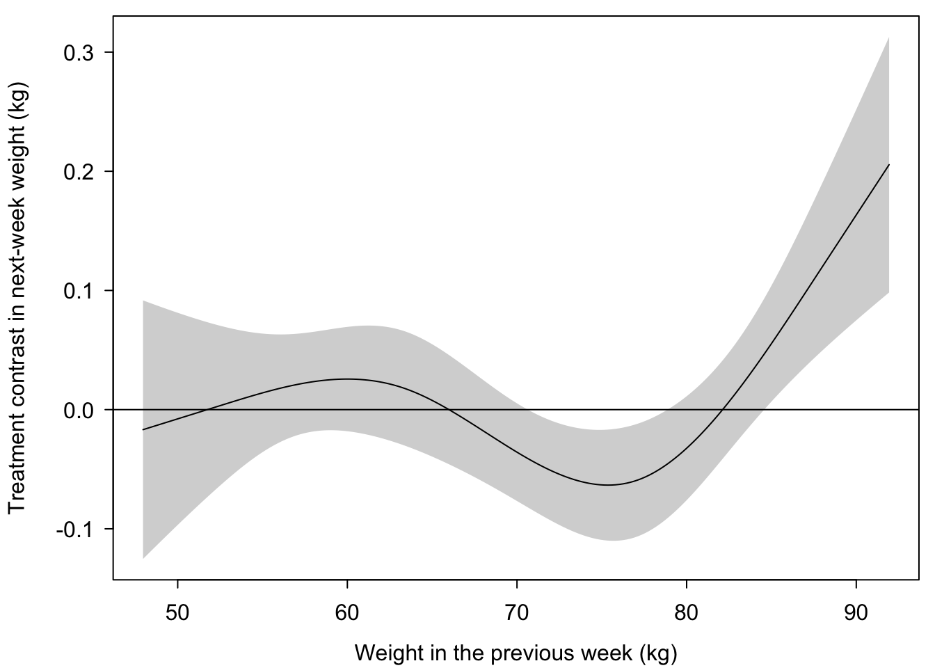
The source is survivor selection that the model does not fully remove. The weight model is fitted only to transitions in which the patient was alive, so it still conditions on survival. Previous and baseline weight absorb most of that selection, but not all of it, because two weights that each vary from week to week do not pin down a patient’s true weight level, and so do not pin down frailty. Where does the remainder show up? For patients whose previous weight is clearly light or clearly heavy, weight already says whether they are frail or robust, and survival selection has nothing left to unbalance. In the middle, between 65 and 75 kg, weight is ambiguous. There the proportion frail among survivors is 0.476 on control and 0.505 on the active treatment, because treatment kept more frail patients alive. Frail patients are lighter, so the active group’s next-week weights are slightly lower in that range. A treatment contrast that is near zero at the extremes and slightly negative in the middle is exactly a treatment × previous weight interaction. Figure 5 shows it in kilograms: within that band the contrast reaches -0.063 kg, at a previous weight of 74.9 kg. Departures near the ends of the weight range reflect the sparseness of data there.

It is not a treatment effect. It is the small remainder of the survivor-selection artifact that previous weight and baseline weight do not fully absorb. Adding the interaction to the model would model the bias, not the biology. The remainder would shrink with more frequent weighing, or with less week-to-week variation, either of which pins down each patient’s true level, and so frailty, more closely.

plt(Contrast ~ yprev, data = ki, ymin = Lower, ymax = Upper,
    type = type_ribbon(),
    xlab = 'Weight in the previous week (kg)',
    ylab = 'Treatment contrast in next-week weight (kg)')
abline(h = 0, lty = 1)

Figure 5: Treatment contrast in mean next-week weight (kg, active minus control) among patients alive in consecutive weeks, as a function of previous weight, for patients whose weight has been stable, from a linear model with the same terms as the interaction model, with 0.95 confidence band. Treatment has no effect on any patient’s weight. Between 65 and 75 kg, where previous weight is least informative about frailty, the contrast reaches -0.063 kg at 74.9 kg.

Death

ws <- seq(50, 95, length = 200)
k  <- contrast(fd,
               list(tx = 1, yprev = ws, wt0 = ws, week = round(m / 2)),
               list(tx = 0, yprev = ws, wt0 = ws, week = round(m / 2)),
               expand = FALSE)
k  <- k[.q(yprev, Contrast, Lower, Upper)]

##  True weekly hazard ratios implied by psurv, for the reference lines
hrtrue <- log(psurv[, 'active']) / log(psurv[, 'control'])

##  Weight at which the estimated treatment odds ratio crosses 1
res$cross <- uniroot(approxfun(k$yprev, k$Contrast), range(k$yprev))$root

cap_gradient <- paste0(
  'Treatment odds ratio for death in the following week as a function of ',
  'weight in the previous week, from the first-order Markov logistic ',
  'transition model, with 0.95 confidence band. The solid line marks no ',
  'effect; the dashed lines are the true weekly hazard ratios built into the ',
  'simulation, ', rnd(hrtrue['frail']), ' for frail patients and ',
  rnd(hrtrue['robust']), ' for robust ones. The model recovers both without ',
  'ever observing frailty, crossing 1.0 at ', round(res$cross, 1),
  ' kg, close to the midpoint (', mean(wlev), ' kg) between the frail and ',
  'robust weight means, where weight no longer discriminates between them. ',
  'Treatment $\\times$ previous weight interaction tests at $\\chi^2$ = ',
  round(res$int_chi, 1), ' on ', res$int_df, ' d.f., P = ', pexp(res$int_p),
  ', while the comparison of survival between treatment groups gives P = ',
  pexp(res$survp), '.')

plt(exp(Contrast) ~ yprev, data = k, ymin = exp(Lower), ymax = exp(Upper),
    type = type_ribbon(), log = 'y',
    xlab = 'Weight in the previous week (kg)',
    ylab = 'Treatment odds ratio for death in the following week')
abline(h = c(hrtrue['frail'], 1, hrtrue['robust']), lty = c(2, 1, 2))

Figure 6: Treatment odds ratio for death in the following week as a function of weight in the previous week, from the first-order Markov logistic transition model, with 0.95 confidence band. The solid line marks no effect; the dashed lines are the true weekly hazard ratios built into the simulation, 0.472 for frail patients and 3.168 for robust ones. The model recovers both without ever observing frailty, crossing 1.0 at 68.8 kg, close to the midpoint (70 kg) between the frail and robust weight means, where weight no longer discriminates between them. Treatment \(\times\) previous weight interaction tests at \(\chi^2\) = 211.8 on 3 d.f., P = \(0\), while the comparison of survival between treatment groups gives P = \(0.98\).

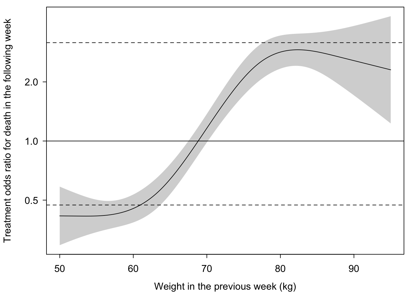
The transition model finds the effect on death that the overall survival comparison could not. Whether treatment raises or lowers the risk of dying depends strongly on how heavy the patient was the week before (\(\chi^2\) = 211.755 on 3 d.f., P = \(0\)). Figure 6 shows the treatment effect as a smooth function of the previous week’s weight. For light patients it settles near the true value for the frail, for heavy patients near the true value for the robust, and it crosses the line of no effect where weight can no longer tell the two kinds apart. The model was never told that there were two kinds of patients; the two levels emerge from the data.

With weekly risks of death this small, odds ratios and hazard ratios for death in a week are nearly equal, so the true weekly hazard ratios are the right reference.

The interaction was not put in the model because the simulation’s truth was known. It belongs there for any analyst who takes the assumption seriously. The assumption says treatment affects no one’s survival, so a check of it must ask whether treatment affects survival in any kind of patient, and whether a treatment effect on death varies with how sick or how heavy a patient is is a central safety question in its own right. Previous weight is the obvious candidate when weight is the outcome under study.

wsel <- c(55, 62, 70, 78, 85)
nd   <- expand.grid(yprev = wsel, tx = 0 : 1, week = round(m / 2))
nd$wt0 <- nd$yprev
nd$lp  <- predict(fd, nd)
ortab  <- data.frame(wsel, exp(nd$lp[nd$tx == 1] - nd$lp[nd$tx == 0]))
names(ortab) <- c('Previous weight (kg)', 'Treatment odds ratio')
knitr::kable(ortab, digits = 2)

Table 3: Estimated treatment odds ratio for death in the following week, for patients whose weight has been stable, so that baseline and previous weight agree.

Previous weight (kg)	Treatment odds ratio
55	0.42
62	0.50
70	1.16
78	2.63
85	2.85

If the assumption that treatment changes no one’s survival is to be relied on at all, this is how it should be checked. If the assumption were true, treatment could have no effect on survival in any group of patients, including groups defined by weight. The transition model examines exactly that. A test of any treatment effect on death, at any previous weight, gives \(\chi^2\) = 211.94 on 4 d.f., P = \(0\), rejecting the assumption decisively in data where the overall survival comparison gives P = \(0.98\).

Given the previous week’s weight, baseline weight is far more informative about next week’s weight (\(\chi^2\) = 62,775 on 3 d.f.) than about death (\(\chi^2\) = 3.381 on 3 d.f.). Predicting next week’s weight benefits from averaging the week-to-week variation of two weights; mortality depends on frailty, for which recent weight is already a good proxy.

The same logic that applied to the overall check applies here. Even a more searching check can only refute the assumption; it can never confirm it, because treatment effects that vary along something leaving no trace in the data would remain invisible. That is the deeper reason not to rely on the assumption at all. The analysis of all patients does not need it: it estimates what treatment did to survival and to weight, among the patients actually randomized, instead of assuming what treatment did not do.

Assumptions That Can Be Checked

The transition models make assumptions too, and an argument for basing inference on data has to say so. What distinguishes them is that every one of them concerns quantities that were observed, so every one can be checked against the data and relaxed if it fails.

• Enough history. The models assume that the previous week’s weight and the baseline weight capture what matters about a patient’s past. Adding the weight from two weeks earlier or the average of all previous weights tests this.
• Non-Markov correlation structure. The Markov structure can be relaxed by adding patient-specific random effects to the model.
• Proportional odds among the living. The weight model assumes that treatment, if it has any effect, shifts the whole distribution of next week’s weight in the same way. This can be checked by comparing treatment odds ratios at different weight cutoffs, and relaxed with a partial proportional odds model. It is assumed only across weights; the death model is a separate binary model with no such assumption.
• Shapes of relationships. Previous and baseline weight enter through flexible splines. Time enters linearly, which a spline in time would test.
• Which effects vary. Whether the effect of treatment on death depends on previous weight was tested directly. The same interaction in the weight model is detectable but tiny, and the expandable note under Weight shows that it reflects leftover survivor selection, not an effect of treatment.
• Overall fit. Combining the transition models gives predicted proportions dead and predicted weight distributions by week and treatment, which can be compared with the observed proportions.

Contrast this with the assumptions behind the survivor analysis: that treatment changes no one’s survival, that it saves but never kills, that membership in an unidentifiable group is predictable from covariates, or any particular way of linking a patient’s two survival outcomes. None of these can be checked in full by any amount of data, because each concerns pairs of outcomes of which at most one is ever seen.

What Formalism Can and Cannot Do

None of this is an argument against careful notation or diagrams. Figure 1 is itself a causal diagram, and it explains in one picture why the survivor comparison fails. Formal tools are good at making assumptions visible and at catching errors of design and analysis before they are made.

What they cannot do is make an assumption true, or make a question answerable when the data cannot answer it. Writing an assumption in precise notation does not make it checkable. Showing that an assumption has some consequence that can be tested does not make the assumption itself testable, especially when the consequence is the weakest one available and is blind to precisely the failure that matters. The precision of the statement is easily mistaken for strength of support, and the more elaborate the machinery, the easier that mistake becomes. Here, careful guidance whose stated purpose is to examine the assumptions behind each analysis describes this assumption as testable. Even if testable is meant only in the narrower sense of falsifiable, readers will naturally take a passed test as support; that is a measure of how easily the mistake is made.

Formal machinery can also change the question without announcing it. “The effect of treatment among patients who would survive on either treatment” sounds like a refinement of the original question, but it is a different question, about a group of patients no one can identify in advance, and a clinician deciding how to treat the patient in front of them cannot use its answer. A related alternative, “the effect that would have been seen if no one had died,” replaces a question about real patients with one about a world that does not exist. Whether always-survivor effects answer a useful question has been debated within the causal inference literature itself (Pearl 2011; VanderWeele 2011); Pearl questioned whether effects defined within principal strata are what a policy or treatment decision needs. Newer separable effects define the target through hypothetical modified treatments instead of unidentifiable groups of patients (Stensrud et al. 2023), at the cost of a different set of untestable assumptions. Analyses of personalized treatment decisions that rely on such unobservable quantities are examined critically by Dawid and Senn (2023). A rigorous formal framework that avoids them altogether, based on decision theory, is described by Dawid (2021) and Constantinou and Dawid (2017).

One simulated trial shows that the offered check can fail completely. It does not show how often it does. But three features of this example are not contrived. The way the two potential outcomes were linked was the one most favorable to the assumption. Treatment effects on survival that go in opposite directions in different kinds of patients are entirely plausible for any treatment with both benefits and safety concerns. Also, trials with such treatments are exactly where an analyst would most want the check to work.

The general principle is that what can be estimated should constrain what is asked. A precisely posed question that the data cannot answer is worth less than an answerable question close to the one the clinician asked. When an outcome such as weight is truncated by death, the clinically sound path is to model all patients, deaths included, and to examine how treatment affects each kind of transition—not to discard the deaths and then assume the consequences away.

Ranking death as the worst outcome is useful for a single overall summary but not required. The separate death and weight transition models used above decouple covariate effects on death from covariate effects on weight, and together make no assumption about where death falls relative to weight.

Summary

When some patients die before an outcome can be measured, a comparison of survivors can show a convincing treatment effect that does not exist, even in a randomized trial. Assuming that treatment changes no patient’s survival repairs the comparison on paper, and equal survival in the two groups is offered as a check. In a simulated trial where the truth is known, and overall survival was identical in the two groups by construction, the check had nothing to detect, while the survivor comparison reported a large, highly significant effect on weight that was entirely an artifact of who survived. No assumption about unobservable quantities could rescue it. What the comparison actually requires is a weaker, more transparent condition whose failure cannot be detected by an overall survival check. A longitudinal ordinal analysis that keeps every patient answers a clinically meaningful question, and modeling the transitions to death separately from changes in weight finds no effect on weight, finds the true effects on survival, and rejects the assumption that the overall check could not. The assumptions these models do make concern only what was observed, and can be checked and relaxed.

Formal machinery is valuable for making assumptions visible, but it gives false comfort when the assumptions cannot be verified or when it quietly substitutes a different question for the one that was asked.

Resources

• ICH E9(R1) addendum on estimands and sensitivity analysis in clinical trials
• Discussion: causal formalism and RCTs
• Causal by design DOI:10.59350/hm05j-h9v33
• Statistical models answer the fundamental clinical question and provide clinical trial estimands DOI:10.59350/rhwfd-tgp07
• Markov longitudinal ordinal models
• General resources for ordinal models

Discussion

To comment or ask questions about this article go to datamethods.org/crct.

Computing Environment

grateful::cite_packages(pkgs = 'Session', output = 'paragraph', out.dir = '.',
    cite.tidyverse = FALSE, omit = c('grateful', 'knitr'))

We used R v. 4.6.1 (R Core Team 2026) and the following R packages: data.table v. 1.18.6.1 (Barrett et al. 2026), Hmisc v. 5.3.1 (Harrell Jr 2026a), rms v. 8.2.2 (Harrell Jr 2026b), tinyplot v. 0.8.0 (McDermott et al. 2026).

The code was run on macOS Golden Gate 27.2.1. It was developed in collaboration with Claude (Anthropic) after extensive interactions.

References

Barrett, Tyson, Matt Dowle, Arun Srinivasan, et al. 2026. data.table: Extension of “data.frame”. https://doi.org/10.32614/CRAN.package.data.table.

Bornkamp, Björn, Kaspar Rufibach, Jianchang Lin, et al. 2021. “Principal Stratum Strategy: Potential Role in Drug Development.” Pharmaceutical Statistics 20 (4): 737–51. https://doi.org/10.1002/pst.2104.

Colantuoni, Elizabeth, Daniel O. Scharfstein, Chenguang Wang, et al. 2018. “Statistical Methods to Compare Functional Outcomes in Randomized Controlled Trials with High Mortality.” BMJ 360 (January): j5748. https://doi.org/10.1136/bmj.j5748.

Constantinou, Panayiota, and A. Philip Dawid. 2017. “Extended Conditional Independence and Applications in Causal Inference.” The Annals of Statistics 45 (6): 2618–53. http://www.jstor.org/stable/26362953.

Dawid, A. P. 2000. “Causal Inference Without Counterfactuals.” Journal of the American Statistical Association 95 (450): 407–24. https://doi.org/10.1080/01621459.2000.10474210.

Dawid, A. Philip, and Stephen Senn. 2023. “Personalised Decision-Making Without Counterfactuals.” Version 2. Pre-published. https://doi.org/10.48550/ARXIV.2301.11976.

Dawid, Philip. 2021. “Decision-Theoretic Foundations for Statistical Causality.” Journal of Causal Inference 9 (1): 39–77. https://doi.org/10.1515/jci-2020-0008.

Ding, Peng, Zhi Geng, Wei Yan, and Xiao-Hua Zhou. 2011. “Identifiability and Estimation of Causal Effects by Principal Stratification With Outcomes Truncated by Death.” Journal of the American Statistical Association 106 (496): 1578–91. https://doi.org/10.1198/jasa.2011.tm10265.

Ding, Peng, and Jiannan Lu. 2017. “Principal Stratification Analysis Using Principal Scores.” Journal of the Royal Statistical Society Series B: Statistical Methodology 79 (3): 757–77. https://doi.org/10.1111/rssb.12191.

Frangakis, Constantine E., and Donald B. Rubin. 2002. “Principal Stratification in Causal Inference.” Biometrics 58 (1): 21–29. https://doi.org/10.1111/j.0006-341X.2002.00021.x.

Harrell, Frank. 2026a. “Causal by Design.” Statistical Thinking, April 8. https://doi.org/10.59350/hm05j-h9v33.

Harrell, Frank. 2026b. “Statistical Models Answer the Fundamental Clinical Question and Provide Clinical Trial Estimands.” Statistical Thinking, July 27. https://doi.org/10.59350/rhwfd-tgp07.

Harrell Jr, Frank E. 2026a. Hmisc: Harrell Miscellaneous. https://hbiostat.org/R/Hmisc/.

Harrell Jr, Frank E. 2026b. rms: Regression Modeling Strategies. https://hbiostat.org/R/rms/.

Hayden, Douglas, Donna K. Pauler, and David Schoenfeld. 2005. “An Estimator for Treatment Comparisons Among Survivors in Randomized Trials.” Biometrics 61: 305–10.

Kahan, Brennan C, Joanna Hindley, Mark Edwards, Suzie Cro, and Tim P Morris. 2024. “The Estimands Framework: A Primer on the ICH E9(R1) Addendum.” BMJ, January 23, e076316. https://doi.org/10.1136/bmj-2023-076316.

Kurland, Brenda F., Laura L. Johnson, Brian L. Engleston, and Paula H. Diehr. 2009. “Longitudinal Data with Follow-up Truncated by Death: Match the Analysis Method to Research Aims.” Stat Sci 24 (2): 211–22.

McDermott, Grant, Vincent Arel-Bundock, and Achim Zeileis. 2026. tinyplot: Lightweight Extension of the Base r Graphics System. https://doi.org/10.32614/CRAN.package.tinyplot.

Pearl, Judea. 2011. “Principal Stratification – a Goal or a Tool?” The International Journal of Biostatistics 7 (1): 1–13. https://doi.org/10.2202/1557-4679.1322.

Pham, Tra My, Brennan C Kahan, Andre Lopes, Memuna Rashid, Peter J Hoskin, and Ian R White. 2025. “Estimating Treatment Effects in Trials with Outcome Data Truncated by Death: A Case Study on Aligning Estimators with Estimands.” Clinical Trials 22 (6): 676–86. https://doi.org/10.1177/17407745251360645.

R Core Team. 2026. R: A Language and Environment for Statistical Computing. R Foundation for Statistical Computing. https://doi.org/10.32614/R.manuals.

Rohde, Maximilian D., Benjamin French, Thomas G. Stewart, and Frank E. Harrell. 2024. “Bayesian Transition Models for Ordinal Longitudinal Outcomes.” Statistics in Medicine 43 (18): 3539–61. https://doi.org/10.1002/sim.10133.

Rubin, Donald B. 1974. “Estimating Causal Effects of Treatments in Randomized and Nonrandomized Studies.” Journal of Educational Psychology 66 (5): 688–701. https://doi.org/10.1037/h0037350.

Rubin, Donald B. 2006. “Causal Inference Through Potential Outcomes and Principal Stratification: Application to Studies with ‘Censoring’ Due to Death.” Statist. Sci. 21 (3): 299–309. https://doi.org/10.1214/088342306000000114.

Senn, Stephen. 2004. “Individual Response to Treatment: Is It a Valid Assumption?” BMJ 329: 966–68.

Senn, Stephen, Katie Rolfe, and Steven A Julious. 2011. “Investigating Variability in Patient Response to Treatment – a Case Study from a Replicate Cross-over Study.” Stat Methods Med Res 20 (6): 657–66. https://doi.org/10.1177/0962280210379174.

Stensrud, Mats J., and Oliver Dukes. 2022. “Translating Questions to Estimands in Randomized Clinical Trials with Intercurrent Events.” Statistics in Medicine n/a (n/a). https://doi.org/10.1002/sim.9398.

Stensrud, Mats J., James M. Robins, Aaron Sarvet, Eric J. Tchetgen Tchetgen, and Jessica G. Young. 2023. “Conditional Separable Effects.” Journal of the American Statistical Association 118 (544): 2671–83. https://doi.org/10.1080/01621459.2022.2071276.

VanderWeele, Tyler J. 2011. “Principal Stratification – Uses and Limitations.” The International Journal of Biostatistics 7 (1): 0000102202155746791329. https://doi.org/10.2202/1557-4679.1329.

Zhang, J. L., and D. B. Rubin. 2003. “Estimation of Causal Effects via Principal Stratification When Some Outcomes Are Truncated by ‘Death’.” J Edu Behav Stat 28: 353–68.