The recent PATH (Predictive Approaches to Treatment effect Heterogeneity) Statement outlines principles, criteria, and key considerations for applying predictive approaches to clinical trials to provide patient-centered evidence in support of decision making. Here challenges in implementing the PATH Statement are addressed with the GUSTO-I trial as a case study.
Department of Biomedical Data Sciences Leiden University Medical Center NL @ESteyerberg
Published
November 24, 2020
Evidence is derived from groups while most medical decisions are made for individual patients. — Kent et al, PATH statement
Heterogeneity of treatment effect (HTE) refers to the nonrandom variation in the magnitude of the absolute treatment effect (treatment benefit) across individual patients. The recent PATH (Predictive Approaches to Treatment effect Heterogeneity) Statement outlines principles, criteria, and key considerations for applying predictive approaches to clinical trials to provide patient-centered evidence in support of decision making. The focus of PATH is on modeling of HTE across individual patients.
The PATH statement lists a number of principles and guidelines. A first principle is to establish overall treatment effect. In another blog, I summarized the arguments in favor of covariate adjustment as the primary analysis of a RCT. Illustration was in the GUSTO-I trial. Here I continue that illustration, also following the blog by Frank Harrell on examining HTE.
Illustration in the GUSTO-I trial
Let’s analyze the data from 30,510 patients with an acute myocardial infarction as included in the GUSTO-I trial. In GUSTO-I, 10,348 patients were randomized to receive tissue plasminogen activator (tPA), while 20,162 were randomzied to Streptokinase (SK) and had 30-day mortality status known.
Code
load(url('http://hbiostat.org/data/repo/gusto.rda'))# keep only SK and tPA arms; and selected set of covariatesgusto <-upData(gusto[gusto$tx=="SK"| gusto$tx=="tPA",], keep=Cs(day30, tx, age, Killip, sysbp, pulse, pmi, miloc, sex),print=FALSE)html(describe(gusto), scroll=TRUE)
gusto Descriptives
gusto
9 Variables 30510 Observations
day30
n
missing
distinct
Info
Sum
Mean
Gmd
30510
0
2
0.195
2128
0.06975
0.1298
sex: Sex
n
missing
distinct
30510
0
2
 Value        male female
 Frequency   22795   7715
 Proportion  0.747  0.253
Killip: Killip Class
n
missing
distinct
30510
0
4
 Value          I    II   III    IV
 Frequency  26007  3857   417   229
 Proportion 0.852 0.126 0.014 0.008
 Value      Inferior    Other Anterior
 Frequency     17582     1062    11866
 Proportion    0.576    0.035    0.389
pmi: Previous MI
n
missing
distinct
30510
0
2
 Value         no   yes
 Frequency  25452  5058
 Proportion 0.834 0.166
tx: Tx in 3 groups
n
missing
distinct
30510
0
2
 Value         SK   tPA
 Frequency  20162 10348
 Proportion 0.661 0.339
Overall treatment effect
The primary outcome was 30-day mortality. Among the tPA group, the 30-day mortality was 653/10,348 = 6.3% vs 1475/20,162 = 7.3% in the SK group. This an absolute difference of 1.0%, or an odds ratio of 0.85 [0.78-0.94].
# 'tpa' as 0/1 variable for tPA vs SK treatmentgusto$tx <-droplevels(gusto$tx) # Drop the SK + tPA category which has 0 obsgusto$tpa <-as.numeric(gusto$tx) -1# 0/1 coding for tPA treatmentlabel(gusto$tpa) <-"tPA"levels(gusto$tpa) <-c("SK", "tPA")tab2 <-table(gusto$day30, gusto$tpa)result <-OddsRatio(tab2, conf.level =0.95)names(result) <-c("Odds Ratio", "Lower CI", "Upper CI")kable(as.data.frame(t(result))) %>%kable_styling(full_width=F, position ="left")
The unadjusted odds ratio of 0.853 is a marginal estimate. As explained in the other blog, a lot can be said in favor of conditional estimates, where we adjust for prognostically important baseline characteristics. In line with Califf 1997 and Steyerberg 2000, we consider a prediction model with 6 baseline covariates, including age and Killip class (a measure for ventricular function). Pulse rate is modeled using a linear spline with a knot at 50 beats/minute.
lrm(formula = day30 ~ tpa + age + Killip + pmin(sysbp, 120) +
    lsp(pulse, 50) + pmi + miloc, data = gusto, x = T, maxit = 99)
Model Likelihood
Ratio Test
Discrimination
Indexes
Rank Discrim.
Indexes
Obs 30510
LR χ2 2991.95
R2 0.235
C 0.815
0 28382
d.f. 11
R211,30510 0.093
Dxy 0.631
1 2128
Pr(>χ2) <0.0001
R211,5938.7 0.395
γ 0.631
max |∂log L/∂β| 7×10⁻¹⁰
Brier 0.056
τa 0.082
β
S.E.
Wald Z
Pr(>|Z|)
Intercept
-3.0203
0.7973
-3.79
0.0002
tpa
-0.2080
0.0529
-3.93
<0.0001
age
0.0769
0.0025
31.28
<0.0001
Killip=II
0.6137
0.0589
10.42
<0.0001
Killip=III
1.1610
0.1214
9.57
<0.0001
Killip=IV
1.9213
0.1618
11.87
<0.0001
sysbp
-0.0392
0.0019
-20.33
<0.0001
pulse
-0.0242
0.0159
-1.52
0.1282
pulse'
0.0433
0.0162
2.67
0.0075
pmi=yes
0.4472
0.0562
7.96
<0.0001
miloc=Other
0.2863
0.1347
2.13
0.0335
miloc=Anterior
0.5432
0.0511
10.62
<0.0001
So, we note that the adjusted regression coefficient for tPA was -0.208. The adjusted OR = 0.812.
Let’s check for statistical interaction with
Individual covariates
The linear predictor
Code
## check for interaction# 1. traditional approachg <-lrm(day30 ~ tx * (age + Killip +pmin(sysbp, 120) +lsp(pulse, 50) + pmi + miloc), data=gusto, maxit=100)print(anova(g)) # tx interactions: 10 df, p=0.5720; based on LR test
Wald Statistics for day30
χ2
d.f.
P
tx (Factor+Higher Order Factors)
23.48
11
0.0151
All Interactions
8.53
10
0.5772
age (Factor+Higher Order Factors)
981.65
2
<0.0001
All Interactions
1.60
1
0.2065
Killip (Factor+Higher Order Factors)
281.44
6
<0.0001
All Interactions
1.37
3
0.7131
sysbp (Factor+Higher Order Factors)
412.30
2
<0.0001
All Interactions
0.11
1
0.7369
pulse (Factor+Higher Order Factors)
235.92
4
<0.0001
All Interactions
4.22
2
0.1214
Nonlinear (Factor+Higher Order Factors)
7.37
2
0.0251
pmi (Factor+Higher Order Factors)
64.23
2
<0.0001
All Interactions
0.05
1
0.8233
miloc (Factor+Higher Order Factors)
115.23
4
<0.0001
All Interactions
2.99
2
0.2239
tx × age (Factor+Higher Order Factors)
1.60
1
0.2065
tx × Killip (Factor+Higher Order Factors)
1.37
3
0.7131
tx × sysbp (Factor+Higher Order Factors)
0.11
1
0.7369
tx × pulse (Factor+Higher Order Factors)
4.22
2
0.1214
Nonlinear
0.08
1
0.7784
Nonlinear Interaction : f(A,B) vs. AB
0.08
1
0.7784
tx × pmi (Factor+Higher Order Factors)
0.05
1
0.8233
tx × miloc (Factor+Higher Order Factors)
2.99
2
0.2239
TOTAL NONLINEAR
7.37
2
0.0251
TOTAL INTERACTION
8.53
10
0.5772
TOTAL NONLINEAR + INTERACTION
15.57
11
0.1579
TOTAL
2343.20
21
<0.0001
Code
# 2. PATH statement: linear interaction with linear predictor; baseline risk, so tx=ref, SKlp.no.tx <- f$coefficients[1] +0* f$coefficients[2] + f$x[,-1] %*% f$coefficients[-(1:2)]gusto$lp <-as.vector(lp.no.tx) # add lp to data frameh <-lrm(day30 ~ tx * lp, data=gusto)print(anova(h)) # tx interaction: 1 df, p=0.35; based on Wald statistics
Wald Statistics for day30
χ2
d.f.
P
tx (Factor+Higher Order Factors)
16.24
2
0.0003
All Interactions
0.86
1
0.3526
lp (Factor+Higher Order Factors)
2338.37
2
<0.0001
All Interactions
0.86
1
0.3526
tx × lp (Factor+Higher Order Factors)
0.86
1
0.3526
TOTAL
2342.20
3
<0.0001
So:
The overall test for interaction with the individual covariates is far from statistically significant (p>0.5).
Similarly, the test for interaction with the linear predictor is far from statistically significant (p>0.3).
Conclusion: no interaction needed
We conclude that we may proceed by ignoring any interactions. We have no evidence against the assumption that the overall effect of treatment is applicable to all patients.
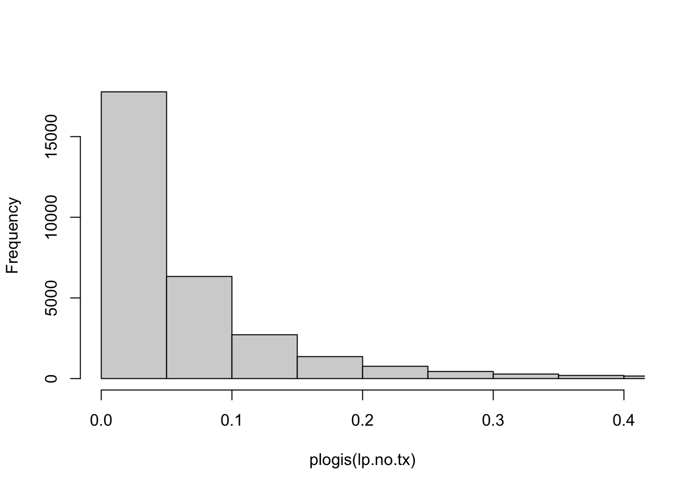
The patients vary widely in risk, as can easily be seen in the histogram below.
Code
hist(plogis(lp.no.tx), xlim=c(0,.4), main="")
We note that many patients have baseline risks (tPA==0) below 5%. Obviously their maximum benefit is bounded by this risk estimate, even if tPA, hypothetically, would reduce the risk to Null.
Reporting RCT results stratified by a risk model is encouraged when overall trial results are positive to better understand the distribution of effects across the trial population.
How do we provide such reporting of RCT results?
We can provide estimates of relative effects and absolute benefit
By group (e.g. quarters defined by quartiles)
By baseline risk (continuous, as in the histogram above)
1a. Relative effects of treatment by risk-group
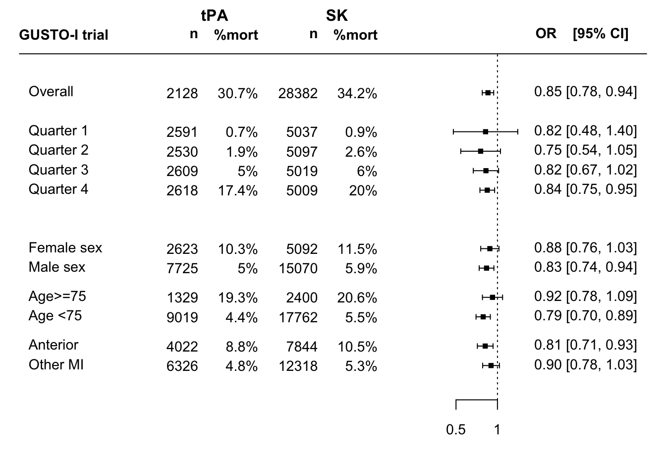
The checks for interaction were far from statistically significant in GUSTO-I. We can further illustrate the relative effects in a forest plot. Many reports from RCTs include forest plots that show relative effects by single variables, such as men vs women; young vs old age; disease subtype; etc.
The PATH statement encourages reporting by risk-based subgroup. How can such reporting be done?
Let’s do some data processing to make a better forest plot.
A PATH compatible forest plot
Let’s expand the standard forest plot for subgroup effects with risk-based subgroups.
Below subgroup effects are defined for 4 risk-based groups using cut2(lp.no.tx, g=4),
and for 3 classical subgroups (by sex, age, type of infarction).
Code
## quantiles, suggest to use quartersgroups <-cut2(lp.no.tx, g=4)group0 <- groups[gusto$tpa==0] # SK gropupgroup1 <- groups[gusto$tpa==1] # tPA grouprate0 <-prop.table(table(group0, gusto$day30[gusto$tpa==0]),1 )[,2]rate1 <-prop.table(table(group1, gusto$day30[gusto$tpa==1]),1 )[,2]ratediff <- rate0-rate1 # benefit of tPA by group# Make a data frame for the resultsdata.subgroups <-as.data.frame(matrix(nrow=(4+6+1), ncol=10))colnames(data.subgroups) <-c("tevent", "tnoevent", "cevent", "cnoevent", "name", "type", "tn", "pt", "cn", "pc")data.subgroups[11,1:4] <-table(gusto$tpa,gusto$day30)[4:1] # overall results# define event and non-event numbersevents1 <-table(group0, gusto$day30[gusto$tpa==0])[,2]nevents1 <-table(group0, gusto$day30[gusto$tpa==0])[,1]events2 <-table(group1, gusto$day30[gusto$tpa==1])[,2]nevents2 <-table(group1, gusto$day30[gusto$tpa==1])[,1]n1 <- events1 + nevents1n2 <- events2 + nevents2data.subgroups[10:7,1:4] <-cbind(events2,nevents2,events1,nevents1)
Data for classic subgroups are managed below:
Code
# Use `table` to get the summary of cell numbers, by subgroup# SEXdata.subgroups[5,1:4] <-table(1-gusto$day30,1-gusto$tpa, gusto$sex)[1:4]data.subgroups[6,1:4] <-table(1-gusto$day30,1-gusto$tpa, gusto$sex)[5:8]# AGEdata.subgroups[3,1:4] <-table(1-gusto$day30,1-gusto$tpa, gusto$age>=75)[1:4]data.subgroups[4,1:4] <-table(1-gusto$day30,1-gusto$tpa, gusto$age>=75)[5:8]# ANTdata.subgroups[1,1:4] <-table(1-gusto$day30,1-gusto$tpa, gusto$miloc=="Anterior")[1:4]data.subgroups[2,1:4] <-table(1-gusto$day30,1-gusto$tpa, gusto$miloc=="Anterior")[5:8]# Namesdata.subgroups[11,5] <-"Overall"data.subgroups[10:7,5] <-paste("Quarter",1:4, sep=" ")data.subgroups[5:6,5] <-c("Male sex","Female sex")data.subgroups[3:4,5] <-c("Age <75","Age>=75")data.subgroups[1:2,5] <-c("Other MI","Anterior")# Type of subgroupdata.subgroups[11,6] <-""data.subgroups[10:7,6] <-c(rep("Risk-based subgroups", length(ratediff)))data.subgroups[1:6,6] <-c(rep("Location",2), rep("Age",2), rep("Sex",2))data.subgroups[,7] <- data.subgroups[,1] + data.subgroups[,2]data.subgroups[,8] <-paste(round(100*data.subgroups[,1] / data.subgroups[,7] , 1),"%", sep="")data.subgroups[,9] <- data.subgroups[,3] + data.subgroups[,4]data.subgroups[,10] <-paste(round(100*data.subgroups[,3] / data.subgroups[,9] , 1),"%", sep="")# Show the datakable(as.data.frame((data.subgroups))) %>%kable_styling(full_width=F, position ="left")
tevent
tnoevent
cevent
cnoevent
name
type
tn
pt
cn
pc
301
6025
649
11669
Other MI
Location
6326
4.8%
12318
5.3%
352
3670
826
7018
Anterior
Location
4022
8.8%
7844
10.5%
397
8622
981
16781
Age <75
Age
9019
4.4%
17762
5.5%
256
1073
494
1906
Age>=75
Age
1329
19.3%
2400
20.6%
383
7342
888
14182
Male sex
Sex
7725
5%
15070
5.9%
270
2353
587
4505
Female sex
Sex
2623
10.3%
5092
11.5%
455
2163
1000
4009
Quarter 4
Risk-based subgroups
2618
17.4%
5009
20%
130
2479
300
4719
Quarter 3
Risk-based subgroups
2609
5%
5019
6%
49
2481
130
4967
Quarter 2
Risk-based subgroups
2530
1.9%
5097
2.6%
19
2572
45
4992
Quarter 1
Risk-based subgroups
2591
0.7%
5037
0.9%
653
1475
9695
18687
Overall
2128
30.7%
28382
34.2%
In this table tevent means #events among treated; cevent means #events among non-treated; etc
Results can be plotted with metafor functions:
Code
par(mar=c(4,4,1,2))### fit random-effects model (use slab argument to define "study" labels)res <-rma(ai=tevent, bi=tnoevent, ci=cevent, di=cnoevent, data=data.subgroups, measure="OR",slab=name, method="ML")### set up forest plot (with 2x2 table counts added); rows argument is used### to specify exactly in which rows the outcomes will be plotted)forest(res, xlim=c(-8, 2.5), at=log(c(0.5, 1)), alim=c(log(0.2), log(2)), atransf=exp,ilab=cbind(data.subgroups$tn, data.subgroups$pt, data.subgroups$cn, data.subgroups$pc),ilab.xpos=c(-5,-4,-3,-2), adj=1,cex=.9, ylim=c(0, 19),rows=c(1:2, (4:5)-.5, 6:7, 10:13, 15),xlab="", mlab="", psize=.8, addfit=F)# lines(x=c(-.15, -.15), y=c(0, 17)) ## could add a reference line of the overall treatment effecttext(c(-5,-4,-3,-2, 2.2), 18, c("n", "%mort", "n", "%mort", "OR [95% CI]"), font=2, adj=1, cex=.9)text(-8, 18, c("GUSTO-I trial"), font=2, adj=0, cex=.9)text(c(-4.5,-2.5), 19, c("tPA", "SK"), font=2, adj=1)
Code
# This can be improved
This forest plot shows the unadjusted overall effect of tPA vs SK treatment; risk-based subgroup effects; and traditional one at a time subgroup effects. The latter are to be interpreted with much caution; many false-positive findings may arise.
Q: What R function can assist trialists in their reporting of risk-based subgroups together with classic subgroups?
We can also estimate the same subgroup effects, adjusted for baseline risk.
Code
# function for adjustmentsubgroup.adj <-function(data=gusto, subgroup=gusto$sex) { coef.unadj <-by(data, subgroup, function(x)lrm.fit(y=x$day30, x=x$tpa)$coef[2]) var.unadj <-by(data, subgroup, function(x)lrm.fit(y=x$day30, x=x$tpa)$var[2,2]) coef.adj <-by(data, subgroup, function(x)lrm.fit(y=x$day30, x=x$tpa, offset=x$lp)$coef[2]) var.adj <-by(data, subgroup, function(x)lrm.fit(y=x$day30, x=x$tpa, offset=x$lp)$var[2,2]) result <-cbind(coef.unadj, coef.adj, coef.ratio=coef.adj/coef.unadj, SEunadj=sqrt(var.unadj), SEadj=sqrt(var.adj), SEratio=sqrt(var.adj)/sqrt(var.unadj)) result} # end functionoptions(digits=3)
Overall trial result (un)adjusted
Code
kable(as.data.frame(subgroup.adj(gusto, gusto$tpa>-1))) %>%kable_styling(full_width=F, position ="left")
coef.unadj
coef.adj
coef.ratio
SEunadj
SEadj
SEratio
TRUE
-0.159
-0.208
1.31
0.049
0.053
1.09
Risk-based subgroups
Code
kable(as.data.frame(subgroup.adj(gusto, groups))) %>%kable_styling(full_width=F, position ="left")
coef.unadj
coef.adj
coef.ratio
SEunadj
SEadj
SEratio
[-7.18,-4.01)
-0.199
-0.198
0.993
0.275
0.275
1.00
[-4.01,-3.20)
-0.282
-0.281
0.998
0.169
0.170
1.00
[-3.20,-2.36)
-0.193
-0.187
0.971
0.108
0.108
1.00
[-2.36, 4.70]
-0.170
-0.208
1.219
0.063
0.067
1.07
Classic subgroup: men vs women
Code
kable(as.data.frame(subgroup.adj(gusto, gusto$sex))) %>%kable_styling(full_width=F, position ="left")
coef.unadj
coef.adj
coef.ratio
SEunadj
SEadj
SEratio
male
-0.183
-0.237
1.29
0.063
0.068
1.08
female
-0.127
-0.164
1.29
0.078
0.085
1.10
Classic subgroup: old (>=75) vs younger age
Code
kable(as.data.frame(subgroup.adj(gusto, gusto$age>=75))) %>%kable_styling(full_width=F, position ="left")
coef.unadj
coef.adj
coef.ratio
SEunadj
SEadj
SEratio
FALSE
-0.239
-0.262
1.1
0.061
0.065
1.06
TRUE
-0.083
-0.100
1.2
0.086
0.093
1.08
The unadjusted and adjusted results are usually quite in line; only subtle differences is the estimates of the relative effects are noted. We might hypothesize that the unadjusted effect for women is confounded by the higher age of women (where higher age was associated with a somewhat weaker treatment effect); this was not confirmed.
Q: What R function can be developed that extends the unadjusted forest plots to provide subgroup effects, adjusted for baseline characteristics?
1b. Absolute benefit of treatment by risk-group
Code
# 95% CI CI <-BinomDiffCI(x1 = events1, n1 = n1, x2 = events2, n2 = n2, method ="scorecc")colnames(CI) <-c("Absolute difference", "Lower CI", "Upper CI")rownames(CI) <-names(events1)result <-round(CI, 3) # absolute difference with confidence intervalkable(as.data.frame(result)) %>%kable_styling(full_width=F, position ="left")
Absolute difference
Lower CI
Upper CI
[-7.18,-4.01)
0.002
-0.003
0.006
[-4.01,-3.20)
0.006
-0.001
0.013
[-3.20,-2.36)
0.010
-0.001
0.020
[-2.36, 4.70]
0.026
0.007
0.044
So, we see a substantial difference in absolute benefit. Low risk according to the linear predictor (lp<-2.36) implies low benefit (<1%); higher risk, higher benefit (>2%). As Frank Harrell would also emphasize, the grouping in quarters might primarily be considered for illustration. A better estimation of benefit avoids grouping, and conditions on the baseline risk.
2a. Relative effects of treatment by baseline risk
The checks for interaction with the linear predictor were far from statistically significant in GUSTO-I, as shown above; supporting the assumption that 1 single adjusted, relative effect applies across baseline risk.
2b. Absolute benefit of treatment by baseline risk
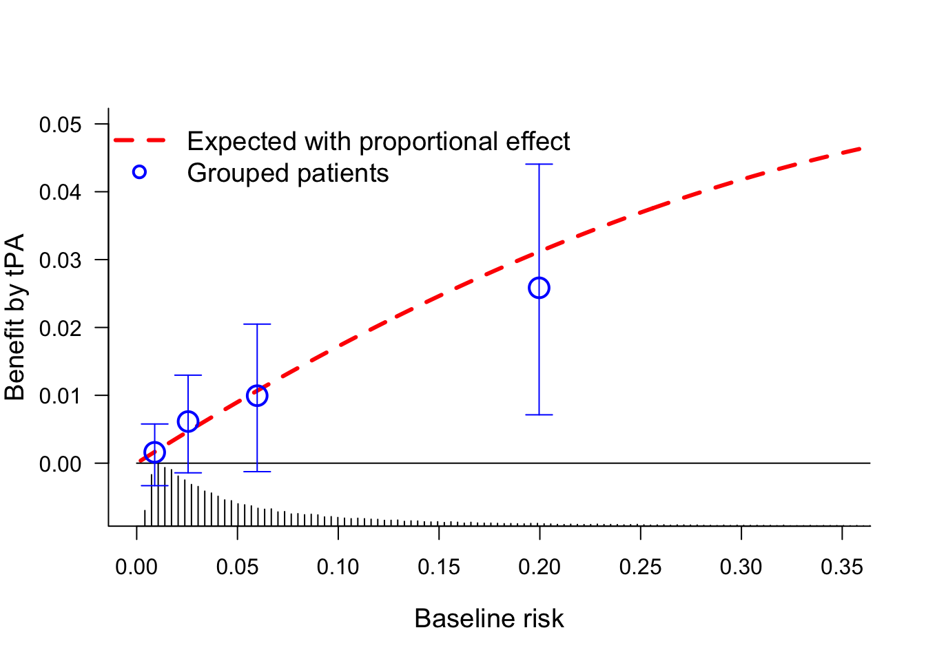
Estimation of absolute benefit can follow a parametric approach, i.e. following the no interaction, main effect model that includes baseline characteristics and a treatment effect; the model f considered above for the primary analysis of the trial.
Further down we will consider relaxations of the proportionality of effect that is assumed in this model.
This plot shows the benefit by tPA treatment over SK. The red line assumes a proportional effect of treatment, which may be quite reasonable here and in many other diseases. The quarters provide for a non-parametric confirmation of the benefit across baseline risk.
Relaxation of the proportional effect assumption
If we want to relax the proportional effect assumption, the blog by Frank Harrell on examining HTE provides an illustration with penalized logistic regression.
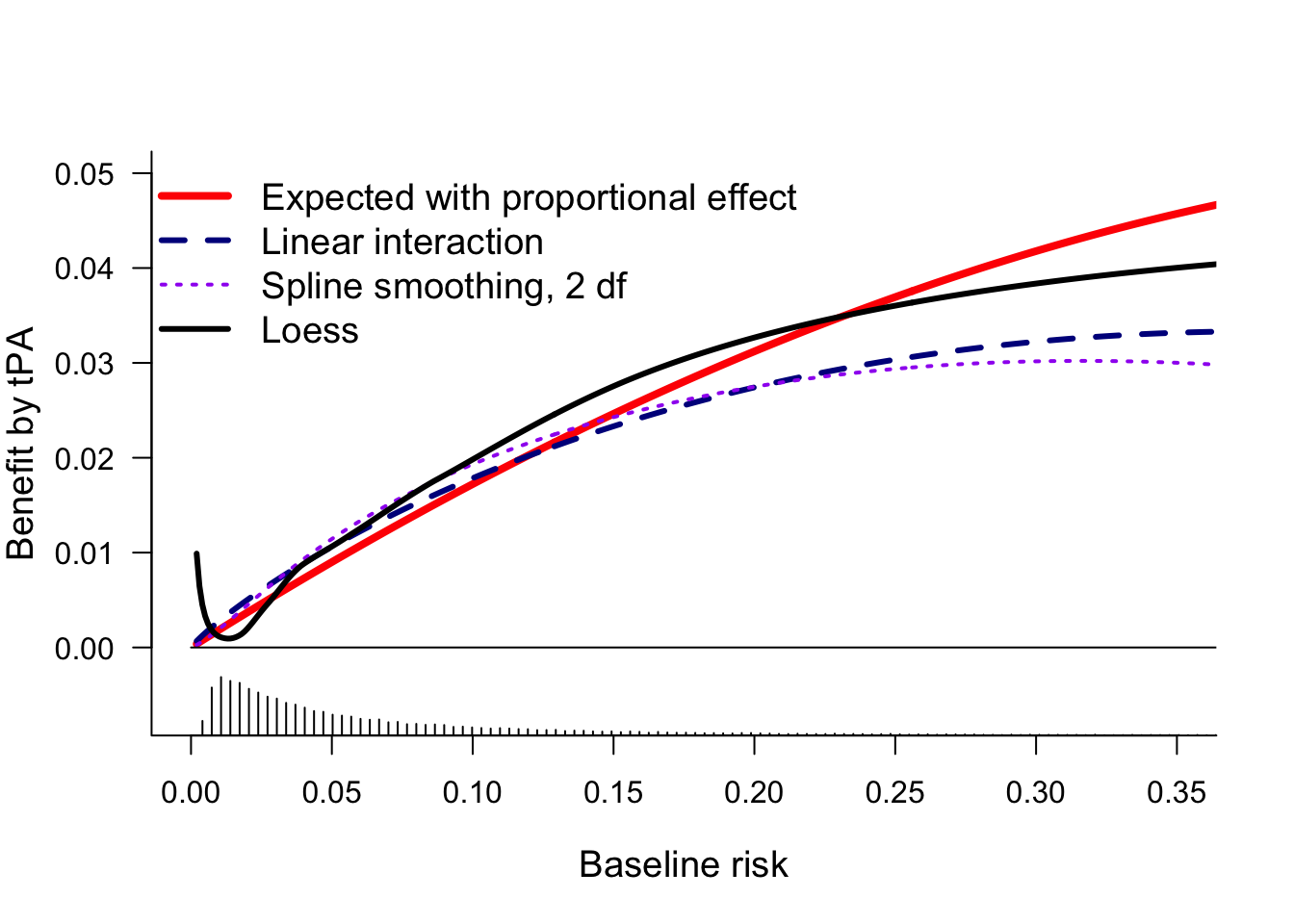
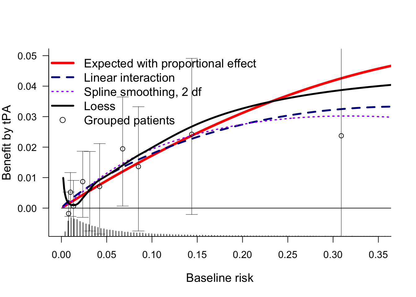
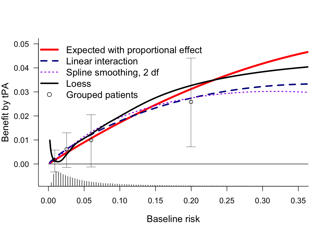
Another possible relaxation is by including interaction with the linear predictor. We consider linear interaction and a non-linear interaction (rcs, 2 df for non-linearity).
And we could try a more non-paramteric approach as in Califf 1997. There, loess smoothers were used for risk estimation the tPA (day30~lp, subset=tpa==1) and SK groups (day30~lp, subset=tpa==0).
Benefit was the differences between these 2 risk groups conditional on baseline risk.
This plot confirms that all estimates of benefit by baseline risk are more or less similar, with benefit clearly increasing by baseline risk. For very low baseline risk, the loess estimates are implausible.
We can also add the grouped observations by decile, as in Califf 1997. The 95% confidence intervals show that the uncertainty per risk group is huge.
Q: How many risk-based groups should be used for illustration of benefit by risk? Default: use quartiles to define 4 quarters; perhaps 3 or only 2 groups in smaller trials?
The GUSTO-I trial serves well to illustrate the impact of conditioning on baseline covariates when we consider relative and absolute effects of treatment on binary outcomes. The risk-adjusted estimate of the overall treatment effect has a different interpretation than the unadjusted estimate: the effect for ‘Patients with acute MI’ versus ‘A patient with a certain risk profile’.
Implications for reporting of RCTs
RCTs typically report on:
an overall effect in the primary analysis;
this analysis should condition on baseline covariates as argued in another blog.
effects stratified by single characteristics: one at a time subgroup analyses;
these analyses should be regarded as secondary and exploratory.
Future RCT reports should include:
an adjusted estimate of the overall treatment effect as the primary analysis;
effects stratified by baseline risk;
typically in 4 risk-based subgroups for illustration,
and in an analysis with continuous baseline risk, typically plotted as benefit by baseline risk.
traditional subgroup analyses only as secondary and exploratory information; not to influence decision-making based on the current RCT, but to inform future studies and new RCTs. An exception may be the situation that strong prior hypotheses exist on effect modeification on the relative scale, as discussed in the ICEMAN report.
The Predictive Approaches to Treatment effect Heterogeneity (PATH) Statement David M. Kent, MD, MS; Jessica K. Paulus, ScD; David van Klaveren, PhD; Ralph D’Agostino, PhD; Steve Goodman, MD, MHS, PhD; Rodney Hayward, MD; John P.A. Ioannidis, MD, DSc; Bray Patrick-Lake, MFS; Sally Morton, PhD; Michael Pencina, PhD; Gowri Raman, MBBS, MS; Joseph S. Ross, MD, MHS; Harry P. Selker, MD, MSPH; Ravi Varadhan, PhD; Andrew Vickers, PhD; John B. Wong, MD; and Ewout W. Steyerberg, PhD Ann Intern Med. 2020;172:35-45.
---title: Implementation of the PATH Statementauthor: - name: Ewout Steyerberg affiliation: Department of Biomedical Data Sciences<br>Leiden University Medical Center NL<br>`@ESteyerberg` url: https://scholar.google.com/citations?user=_75LDyMAAAAJ&hl=nl email: e.w.steyerberg@lumc.nldate: 2020-11-24contents: [RCT, drug-evaluation, generalizability, medicine, personalized-medicine, prediction, subgroup, 2020]description: 'The recent PATH (Predictive Approaches to Treatment effect Heterogeneity) Statement outlines principles, criteria, and key considerations for applying predictive approaches to clinical trials to provide patient-centered evidence in support of decision making. Here challenges in implementing the PATH Statement are addressed with the GUSTO-I trial as a case study.'---```{r setup, include=FALSE}require(rms)require(table1)require(DescTools)require(metafor)require(knitr)require(kableExtra)options(digits=3)mu <- markupSpecs$html # in Hmisc```::: {.quoteit}Evidence is derived from groups while most medical decisions are made for individual patients. — Kent _et al_, PATH statement:::Heterogeneity of treatment effect (**_HTE_**) refers to the nonrandom variation in the magnitude of the absolute treatment effect (**_treatment benefit_**) across individual patients. The recent **_[PATH](https://www.ncbi.nlm.nih.gov/pubmed/31711134)_** (Predictive Approaches to Treatment effect Heterogeneity) Statement outlines principles, criteria, and key considerations for applying predictive approaches to clinical trials to provide patient-centered evidence in support of decision making. The focus of PATH is on modeling of **_HTE_** across individual patients. [[Comments](https://hbiostat.org/comment.html)]{.aside}The PATH statement lists a number of principles and guidelines. A first principle is to establish **_overall treatment effect_**. In another [blog](../covadj), I summarized the arguments in favor of covariate adjustment as the primary analysis of a RCT. Illustration was in the GUSTO-I trial. Here I continue that illustration, also following the blog by **Frank Harrell** on **_[examining HTE](../varyor)_**.## Illustration in the GUSTO-I trialLet's analyze the data from 30,510 patients with an acute myocardial infarction as included in the GUSTO-I trial. In GUSTO-I, 10,348 patients were randomized to receive tissue plasminogen activator (tPA), while 20,162 were randomzied to Streptokinase (SK) and had 30-day mortality status known.```{r IDA.gusto}load(url('http://hbiostat.org/data/repo/gusto.rda'))# keep only SK and tPA arms; and selected set of covariatesgusto <-upData(gusto[gusto$tx=="SK"| gusto$tx=="tPA",], keep=Cs(day30, tx, age, Killip, sysbp, pulse, pmi, miloc, sex),print=FALSE)html(describe(gusto), scroll=TRUE)```### Overall treatment effectThe primary outcome was 30-day mortality. Among the tPA group, the 30-day mortality was 653/10,348 = 6.3% vs 1475/20,162 = 7.3% in the SK group. This an absolute difference of 1.0%, or an odds ratio of 0.85 [0.78-0.94].```{r overall.tx}# simple cross-tabletable1(~as.factor(day30) | tx, data=gusto, digits=2) # 'tpa' as 0/1 variable for tPA vs SK treatmentgusto$tx <-droplevels(gusto$tx) # Drop the SK + tPA category which has 0 obsgusto$tpa <-as.numeric(gusto$tx) -1# 0/1 coding for tPA treatmentlabel(gusto$tpa) <-"tPA"levels(gusto$tpa) <-c("SK", "tPA")tab2 <-table(gusto$day30, gusto$tpa)result <-OddsRatio(tab2, conf.level =0.95)names(result) <-c("Odds Ratio", "Lower CI", "Upper CI")kable(as.data.frame(t(result))) %>%kable_styling(full_width=F, position ="left")# BinomDiffCI(x1 = events1, n1 = n1, x2 = events2, n2 = n2, ...)CI <-BinomDiffCI(x1 = tab2[2,1], n1 =sum(tab2[,1]), x2 = tab2[2,2], n2 =sum(tab2[,2]),method ="scorecc")colnames(CI) <-c("Absolute difference", "Lower CI", "Upper CI")result <-round(CI, 3) # absolute difference with confidence intervalkable(as.data.frame(result)) %>%kable_styling(full_width=F, position ="left")```***### Adjustment for baseline covariatesThe unadjusted odds ratio of `r round(OddsRatio(tab2, conf.level = 0.95)[1], 3)` is a marginal estimate. As explained in the other blog, a lot can be said in favor of *conditional estimates*, where we adjust for prognostically important baseline characteristics. In line with [Califf 1997](https://www.sciencedirect.com/science/article/pii/S0002870397701649) and [Steyerberg 2000](https://www.sciencedirect.com/science/article/pii/S0002870300900012), we consider a prediction model with 6 baseline covariates, including age and Killip class (a measure for ventricular function). Pulse rate is modeled using a linear spline with a knot at 50 beats/minute.```{r adjusted.tx}options(prType='html')f <-lrm(day30 ~ tpa + age + Killip +pmin(sysbp, 120) +lsp(pulse, 50) + pmi + miloc, data=gusto, x=T, maxit=99)print(f) # coef tPA: -0.2080```So, we note that the **adjusted** regression coefficient for tPA was `r round(f$coef[2],4)`. The adjusted OR = `r round(exp(f$coef[2]),3)`. Let's check for statistical interaction with1. Individual covariates 2. The linear predictor ```{r interaction.tx}## check for interaction# 1. traditional approachg <-lrm(day30 ~ tx * (age + Killip +pmin(sysbp, 120) +lsp(pulse, 50) + pmi + miloc), data=gusto, maxit=100)print(anova(g)) # tx interactions: 10 df, p=0.5720; based on LR test# 2. PATH statement: linear interaction with linear predictor; baseline risk, so tx=ref, SKlp.no.tx <- f$coefficients[1] +0* f$coefficients[2] + f$x[,-1] %*% f$coefficients[-(1:2)]gusto$lp <-as.vector(lp.no.tx) # add lp to data frameh <-lrm(day30 ~ tx * lp, data=gusto)print(anova(h)) # tx interaction: 1 df, p=0.35; based on Wald statistics```So: 1. The overall test for interaction with the individual covariates is far from statistically significant (p>0.5). 2. Similarly, the test for interaction with the linear predictor is far from statistically significant (p>0.3). #### Conclusion: no interaction neededWe conclude that we may proceed by ignoring any interactions. We have no evidence against the assumption that the overall effect of treatment is applicable to all patients. The patients vary widely in risk, as can easily be seen in the histogram below. ```{r histogram.lp}hist(plogis(lp.no.tx), xlim=c(0,.4), main="")```We note that many patients have baseline risks (tPA==0) below 5%. Obviously their maximum benefit is bounded by this risk estimate, even if tPA, hypothetically, would reduce the risk to Null.## PATH principle: perform risk-based subgrouping**_[Fig 3](https://www.ncbi.nlm.nih.gov/pubmed/31711134)_** of the PATH Statement starts with: ::: {.quoteit}Reporting RCT results stratified by a risk model is encouraged when overall trial results are positive to better understand the distribution of effects across the trial population.:::How do we provide such reporting of RCT results? We can provide estimates of relative effects and absolute benefit1. By group (e.g. quarters defined by quartiles) 2. By baseline risk (continuous, as in the histogram above) ### 1a. Relative effects of treatment by risk-groupThe checks for interaction were far from statistically significant in GUSTO-I. We can further illustrate the relative effects in a forest plot. Many reports from RCTs include forest plots that show relative effects by single variables, such as men vs women; young vs old age; disease subtype; etc. The *PATH* statement encourages reporting by risk-based subgroup. How can such reporting be done? Let's do some data processing to make a better forest plot.#### A PATH compatible forest plotLet's expand the standard forest plot for subgroup effects with risk-based subgroups. Below subgroup effects are defined for 4 risk-based groups using `cut2(lp.no.tx, g=4)`, and for 3 classical subgroups (by sex, age, type of infarction). ```{r risk.subgroup.effects}## quantiles, suggest to use quartersgroups <-cut2(lp.no.tx, g=4)group0 <- groups[gusto$tpa==0] # SK gropupgroup1 <- groups[gusto$tpa==1] # tPA grouprate0 <-prop.table(table(group0, gusto$day30[gusto$tpa==0]),1 )[,2]rate1 <-prop.table(table(group1, gusto$day30[gusto$tpa==1]),1 )[,2]ratediff <- rate0-rate1 # benefit of tPA by group# Make a data frame for the resultsdata.subgroups <-as.data.frame(matrix(nrow=(4+6+1), ncol=10))colnames(data.subgroups) <-c("tevent", "tnoevent", "cevent", "cnoevent", "name", "type", "tn", "pt", "cn", "pc")data.subgroups[11,1:4] <-table(gusto$tpa,gusto$day30)[4:1] # overall results# define event and non-event numbersevents1 <-table(group0, gusto$day30[gusto$tpa==0])[,2]nevents1 <-table(group0, gusto$day30[gusto$tpa==0])[,1]events2 <-table(group1, gusto$day30[gusto$tpa==1])[,2]nevents2 <-table(group1, gusto$day30[gusto$tpa==1])[,1]n1 <- events1 + nevents1n2 <- events2 + nevents2data.subgroups[10:7,1:4] <-cbind(events2,nevents2,events1,nevents1)```Data for classic subgroups are managed below: ```{r classic.subgroup.effects}# Use `table` to get the summary of cell numbers, by subgroup# SEXdata.subgroups[5,1:4] <-table(1-gusto$day30,1-gusto$tpa, gusto$sex)[1:4]data.subgroups[6,1:4] <-table(1-gusto$day30,1-gusto$tpa, gusto$sex)[5:8]# AGEdata.subgroups[3,1:4] <-table(1-gusto$day30,1-gusto$tpa, gusto$age>=75)[1:4]data.subgroups[4,1:4] <-table(1-gusto$day30,1-gusto$tpa, gusto$age>=75)[5:8]# ANTdata.subgroups[1,1:4] <-table(1-gusto$day30,1-gusto$tpa, gusto$miloc=="Anterior")[1:4]data.subgroups[2,1:4] <-table(1-gusto$day30,1-gusto$tpa, gusto$miloc=="Anterior")[5:8]# Namesdata.subgroups[11,5] <-"Overall"data.subgroups[10:7,5] <-paste("Quarter",1:4, sep=" ")data.subgroups[5:6,5] <-c("Male sex","Female sex")data.subgroups[3:4,5] <-c("Age <75","Age>=75")data.subgroups[1:2,5] <-c("Other MI","Anterior")# Type of subgroupdata.subgroups[11,6] <-""data.subgroups[10:7,6] <-c(rep("Risk-based subgroups", length(ratediff)))data.subgroups[1:6,6] <-c(rep("Location",2), rep("Age",2), rep("Sex",2))data.subgroups[,7] <- data.subgroups[,1] + data.subgroups[,2]data.subgroups[,8] <-paste(round(100*data.subgroups[,1] / data.subgroups[,7] , 1),"%", sep="")data.subgroups[,9] <- data.subgroups[,3] + data.subgroups[,4]data.subgroups[,10] <-paste(round(100*data.subgroups[,3] / data.subgroups[,9] , 1),"%", sep="")# Show the datakable(as.data.frame((data.subgroups))) %>%kable_styling(full_width=F, position ="left")```In this table **tevent** means #events among treated; **cevent** means #events among non-treated; etc Results can be plotted with `metafor` functions: ```{r subgroup.effects}par(mar=c(4,4,1,2))### fit random-effects model (use slab argument to define "study" labels)res <-rma(ai=tevent, bi=tnoevent, ci=cevent, di=cnoevent, data=data.subgroups, measure="OR",slab=name, method="ML")### set up forest plot (with 2x2 table counts added); rows argument is used### to specify exactly in which rows the outcomes will be plotted)forest(res, xlim=c(-8, 2.5), at=log(c(0.5, 1)), alim=c(log(0.2), log(2)), atransf=exp,ilab=cbind(data.subgroups$tn, data.subgroups$pt, data.subgroups$cn, data.subgroups$pc),ilab.xpos=c(-5,-4,-3,-2), adj=1,cex=.9, ylim=c(0, 19),rows=c(1:2, (4:5)-.5, 6:7, 10:13, 15),xlab="", mlab="", psize=.8, addfit=F)# lines(x=c(-.15, -.15), y=c(0, 17)) ## could add a reference line of the overall treatment effecttext(c(-5,-4,-3,-2, 2.2), 18, c("n", "%mort", "n", "%mort", "OR [95% CI]"), font=2, adj=1, cex=.9)text(-8, 18, c("GUSTO-I trial"), font=2, adj=0, cex=.9)text(c(-4.5,-2.5), 19, c("tPA", "SK"), font=2, adj=1)# This can be improved```This forest plot shows the unadjusted overall effect of tPA vs SK treatment; risk-based subgroup effects; and traditional one at a time subgroup effects. The latter are to be interpreted with much caution; many false-positive findings may arise. ::: {.quoteit}Q: What R function can assist trialists in their reporting of risk-based subgroups together with classic subgroups?:::We can also estimate the same subgroup effects, adjusted for baseline risk.```{r adjusted.subgroup.effects.function}# function for adjustmentsubgroup.adj <-function(data=gusto, subgroup=gusto$sex) { coef.unadj <-by(data, subgroup, function(x)lrm.fit(y=x$day30, x=x$tpa)$coef[2]) var.unadj <-by(data, subgroup, function(x)lrm.fit(y=x$day30, x=x$tpa)$var[2,2]) coef.adj <-by(data, subgroup, function(x)lrm.fit(y=x$day30, x=x$tpa, offset=x$lp)$coef[2]) var.adj <-by(data, subgroup, function(x)lrm.fit(y=x$day30, x=x$tpa, offset=x$lp)$var[2,2]) result <-cbind(coef.unadj, coef.adj, coef.ratio=coef.adj/coef.unadj, SEunadj=sqrt(var.unadj), SEadj=sqrt(var.adj), SEratio=sqrt(var.adj)/sqrt(var.unadj)) result} # end functionoptions(digits=3)```Overall trial result (un)adjusted```{r}kable(as.data.frame(subgroup.adj(gusto, gusto$tpa>-1))) %>%kable_styling(full_width=F, position ="left")```Risk-based subgroups```{r}kable(as.data.frame(subgroup.adj(gusto, groups))) %>%kable_styling(full_width=F, position ="left")```Classic subgroup: men vs women```{r}kable(as.data.frame(subgroup.adj(gusto, gusto$sex))) %>%kable_styling(full_width=F, position ="left")```Classic subgroup: old (>=75) vs younger age```{r}kable(as.data.frame(subgroup.adj(gusto, gusto$age>=75))) %>%kable_styling(full_width=F, position ="left")```The unadjusted and adjusted results are usually quite in line; only subtle differences is the estimates of the relative effects are noted. We might hypothesize that the unadjusted effect for women is confounded by the higher age of women (where higher age was associated with a somewhat weaker treatment effect); this was not confirmed. ::: {.quoteit}Q: What R function can be developed that extends the unadjusted forest plots to provide subgroup effects, adjusted for baseline characteristics?:::### 1b. Absolute benefit of treatment by risk-group ```{r grouping}# 95% CI CI <-BinomDiffCI(x1 = events1, n1 = n1, x2 = events2, n2 = n2, method ="scorecc")colnames(CI) <-c("Absolute difference", "Lower CI", "Upper CI")rownames(CI) <-names(events1)result <-round(CI, 3) # absolute difference with confidence intervalkable(as.data.frame(result)) %>%kable_styling(full_width=F, position ="left")```So, we see a substantial difference in absolute benefit. Low risk according to the linear predictor (lp<-2.36) implies low benefit (<1%); higher risk, higher benefit (>2%). As **Frank Harrell** would also emphasize, the grouping in quarters might primarily be considered for illustration. A better estimation of benefit avoids grouping, and conditions on the baseline risk. ### 2a. Relative effects of treatment by baseline riskThe checks for interaction with the linear predictor were far from statistically significant in GUSTO-I, as shown above; supporting the assumption that 1 single adjusted, relative effect applies across baseline risk. ### 2b. Absolute benefit of treatment by baseline riskEstimation of absolute benefit can follow a parametric approach, i.e. following the no interaction, main effect model that includes baseline characteristics and a treatment effect; the model `f` considered above for the primary analysis of the trial. Further down we will consider relaxations of the proportionality of effect that is assumed in this model.```{r plot.benefit}# create baseline predictions: X-axisxp <-seq(0.002,.5,by=0.001)logxp0 <-log(xp/(1-xp))# expected difference, if covariate adjusted model holdsp1exp <-plogis(logxp0) -plogis(logxp0+coef(f)[2]) # proportional effect assumedplot(x=xp, y=p1exp, type='l', lty=2, lwd=3, xlim=c(0,.35), ylim=c(-0.007,.05), col="red",xlab="Baseline risk", ylab="Benefit by tPA", cex.lab=1.2, las=1, bty='l' )# add horizontal linelines(x=c(0,.5), y=c(0,0)) # distribution of predicted histSpike(plogis(lp.no.tx), add=T, side=1, nint=300, frac=.15) points(x=rate0, y=ratediff, pch=1, cex=2, lwd=2, col="blue")arrows(x0=rate0, x1=rate0, y0=CI[,2], y1=CI[,3], angle=90, code=3,len=.1, col="blue")legend("topleft", lty=c(2,NA), pch=c(NA,1), lwd=c(3,2), bty='n',col=c("red", "blue"), cex=1.2,legend=c("Expected with proportional effect", "Grouped patients"))```This plot shows the benefit by tPA treatment over SK. The red line assumes a proportional effect of treatment, which may be quite reasonable here and in many other diseases. The quarters provide for a non-parametric confirmation of the benefit across baseline risk. ### Relaxation of the proportional effect assumptionIf we want to relax the proportional effect assumption, the blog by **Frank Harrell** on **_[examining HTE](../varyor/)_** provides an illustration with **penalized logistic regression**.Another possible relaxation is by including **interaction with the linear predictor**. We consider linear interaction and a non-linear interaction (`rcs`, 2 *df* for non-linearity). And we could try a more non-paramteric approach as in [Califf 1997](https://www.sciencedirect.com/science/article/pii/S0002870397701649). There, `loess` smoothers were used for risk estimation the tPA (`day30~lp, subset=tpa==1`) and SK groups (`day30~lp, subset=tpa==0`). Benefit was the differences between these 2 risk groups conditional on baseline risk.```{r interaction.with.lp}h <-lrm(day30 ~ tpa + tpa * lp, data=gusto, eps=0.005, maxit=30)h2 <-lrm(day30 ~ tpa +rcs(lp,3)*tpa, data=gusto, eps=0.005, maxit=99)# loess smoothingl0 <-loess(day30 ~ lp, data=gusto, subset=tpa==0)l1 <-loess(day30 ~ lp, data=gusto, subset=tpa==1)# subtract predicted risks with from without txp1 <-plogis(Predict(h, tpa=0, lp = logxp0)[,3]) -plogis(Predict(h, tpa=1, lp = logxp0)[,3])p2 <-plogis(Predict(h2, tpa=0, lp = logxp0)[,3]) -plogis(Predict(h2, tpa=1, lp = logxp0)[,3])l <-predict(l0, data.frame(lp = logxp0)) -predict(l1, data.frame(lp = logxp0))plot(x=xp, y=p1exp, type='l', lty=1, lwd=4, xlim=c(0,.35), ylim=c(-0.007,.05), col="red",xlab="Baseline risk", ylab="Benefit by tPA", cex.lab=1.2, las=1, bty='l' )# benefit with interaction termslines(x=xp, y=p1, type='l', lty=2, lwd=3, col="dark blue") lines(x=xp, y=p2, type='l', lty=3, lwd=2, col="purple") lines(x=xp, y=l, type='l', lty=1, lwd=3, col="black") # horizontal linelines(x=c(0,.5), y=c(0,0)) # distribution of predicted histSpike(plogis(lp.no.tx), add=T, side=1, nint=300, frac=.1) legend("topleft", lty=c(1,2,3,1), pch=c(NA,NA,NA,NA), lwd=c(4,3,2,3), bty='n',col=c("red", "dark blue", "purple","black"), cex=1.2,legend=c("Expected with proportional effect", "Linear interaction", "Spline smoothing, 2 df","Loess"))```This plot confirms that all estimates of benefit by baseline risk are more or less similar, with benefit clearly increasing by baseline risk. For very low baseline risk, the `loess` estimates are implausible. We can also add the grouped observations by decile, as in [Califf 1997](https://www.sciencedirect.com/science/article/pii/S0002870397701649). The 95% confidence intervals show that the uncertainty per risk group is huge.::: {.quoteit}Q: How many risk-based groups should be used for illustration of benefit by risk? Default: use quartiles to define 4 quarters; perhaps 3 or only 2 groups in smaller trials?:::```{r interaction.with.lp.deciles}g <-10# first decilesh <-lrm(day30 ~ tpa + tpa * lp, data=gusto, eps=0.005, maxit=30)h2 <-lrm(day30 ~ tpa +rcs(lp,3)*tpa, data=gusto, eps=0.005, maxit=99)# loess smoothingl0 <-loess(day30 ~ lp, data=gusto, subset=tpa==0)l1 <-loess(day30 ~ lp, data=gusto, subset=tpa==1)# subtract predicted risks with from without txp1 <-plogis(Predict(h, tpa=0, lp = logxp0)[,3]) -plogis(Predict(h, tpa=1, lp = logxp0)[,3])p2 <-plogis(Predict(h2, tpa=0, lp = logxp0)[,3]) -plogis(Predict(h2, tpa=1, lp = logxp0)[,3])l <-predict(l0, data.frame(lp = logxp0)) -predict(l1, data.frame(lp = logxp0))plot(x=xp, y=p1exp, type='l', lty=1, lwd=4, xlim=c(0,.35), ylim=c(-0.007,.05), col="red",xlab="Baseline risk", ylab="Benefit by tPA", cex.lab=1.2, las=1, bty='l' )# benefit with interaction termslines(x=xp, y=p1, type='l', lty=2, lwd=3, col="dark blue") lines(x=xp, y=p2, type='l', lty=3, lwd=2, col="purple") lines(x=xp, y=l, type='l', lty=1, lwd=3, col="black") # horizontal linelines(x=c(0,.5), y=c(0,0)) # distribution of predicted histSpike(plogis(lp.no.tx), add=T, side=1, nint=300, frac=.1) # risk groupsgroups <-cut2(lp.no.tx, g=g)group0 <- groups[gusto$tpa==0] # SK gropupgroup1 <- groups[gusto$tpa==1] # tPA grouprate0 <-prop.table(table(group0, gusto$day30[gusto$tpa==0]),1 )[,2]rate1 <-prop.table(table(group1, gusto$day30[gusto$tpa==1]),1 )[,2]ratediff <- rate0-rate1 # benefit of tPA by group# CI re-calculationevents1 <-table(group0, gusto$day30[gusto$tpa==0])[,2]nevents1 <-table(group0, gusto$day30[gusto$tpa==0])[,1]events2 <-table(group1, gusto$day30[gusto$tpa==1])[,2]nevents2 <-table(group1, gusto$day30[gusto$tpa==1])[,1]n1 <- events1 + nevents1n2 <- events2 + nevents2CI <-BinomDiffCI(x1 = events1, n1 = n1, x2 = events2, n2 = n2, method ="scorecc")points(x=rate0, y=ratediff, pch=1, cex=1, lwd=1, col="black")arrows(x0=rate0, x1=rate0, y0=CI[,2], y1=CI[,3], angle=90, code=3,len=.1, col="black", lwd=.5)legend("topleft", lty=c(1,2,3,1,NA), pch=c(NA,NA,NA,NA,1), lwd=c(4,3,2,3,1), bty='n',col=c("red", "dark blue", "purple","black","black"), cex=1.2,legend=c("Expected with proportional effect", "Linear interaction", "Spline smoothing, 2 df","Loess","Grouped patients"))``````{r interaction.with.lp.quarters}g <-4# quartersplot(x=xp, y=p1exp, type='l', lty=1, lwd=4, xlim=c(0,.35), ylim=c(-0.007,.05), col="red",xlab="Baseline risk", ylab="Benefit by tPA", cex.lab=1.2, las=1, bty='l' )# benefit with interaction termslines(x=xp, y=p1, type='l', lty=2, lwd=3, col="dark blue") lines(x=xp, y=p2, type='l', lty=3, lwd=2, col="purple") lines(x=xp, y=l, type='l', lty=1, lwd=3, col="black") # horizontal linelines(x=c(0,.5), y=c(0,0)) # distribution of predicted histSpike(plogis(lp.no.tx), add=T, side=1, nint=300, frac=.1) # risk groupsgroups <-cut2(lp.no.tx, g=g)group0 <- groups[gusto$tpa==0] # SK gropupgroup1 <- groups[gusto$tpa==1] # tPA grouprate0 <-prop.table(table(group0, gusto$day30[gusto$tpa==0]),1 )[,2]rate1 <-prop.table(table(group1, gusto$day30[gusto$tpa==1]),1 )[,2]ratediff <- rate0-rate1 # benefit of tPA by group# CI re-calculationevents1 <-table(group0, gusto$day30[gusto$tpa==0])[,2]nevents1 <-table(group0, gusto$day30[gusto$tpa==0])[,1]events2 <-table(group1, gusto$day30[gusto$tpa==1])[,2]nevents2 <-table(group1, gusto$day30[gusto$tpa==1])[,1]n1 <- events1 + nevents1n2 <- events2 + nevents2CI <-BinomDiffCI(x1 = events1, n1 = n1, x2 = events2, n2 = n2, method ="scorecc")points(x=rate0, y=ratediff, pch=1, cex=1, lwd=1, col="black")arrows(x0=rate0, x1=rate0, y0=CI[,2], y1=CI[,3], angle=90, code=3,len=.1, col="black", lwd=.5)legend("topleft", lty=c(1,2,3,1,NA), pch=c(NA,NA,NA,NA,1), lwd=c(4,3,2,3,1), bty='n',col=c("red", "dark blue", "purple","black","black"), cex=1.2,legend=c("Expected with proportional effect", "Linear interaction", "Spline smoothing, 2 df","Loess","Grouped patients"))```## ConclusionsThe GUSTO-I trial serves well to illustrate the impact of conditioning on baseline covariates when we consider relative and absolute effects of treatment on binary outcomes. The risk-adjusted estimate of the overall treatment effect has a different interpretation than the unadjusted estimate: the effect for *‘Patients with acute MI’* versus *‘A patient with a certain risk profile’*. ### Implications for reporting of RCTsRCTs typically report on: 1. an overall effect in the primary analysis; this analysis should condition on baseline covariates as argued in another blog. 2. effects stratified by single characteristics: one at a time subgroup analyses; these analyses should be regarded as secondary and exploratory.Future RCT reports should include: 1. an adjusted estimate of the overall treatment effect as the primary analysis; 2. effects stratified by baseline risk; typically in 4 risk-based subgroups for illustration, and in an analysis with continuous baseline risk, typically plotted as benefit by baseline risk. 3. traditional subgroup analyses only as secondary and exploratory information; not to influence decision-making based on the current RCT, but to inform future studies and new RCTs. An exception may be the situation that strong prior hypotheses exist on effect modeification on the relative scale, as discussed in the [ICEMAN report](https://macsphere.mcmaster.ca/handle/11375/24375).### References#### GUSTO-I referencesGusto Investigators - New England Journal of Medicine, 1993 [An international randomized trial comparing four thrombolytic strategies for acute myocardial infarction](https://www.nejm.org/doi/full/10.1056/NEJM199309023291001)Califf R, …, ML Simoons, EJ Topol, GUSTO-I Investigators - American heart journal, 1997 [Selection of thrombolytic therapy for individual patients: development of a clinical model](https://www.sciencedirect.com/science/article/pii/S0002870397701649)EW Steyerberg, PMM Bossuyt, KL Lee - American heart journal, 2000 [Clinical trials in acute myocardial infarction: should we adjust for baseline characteristics?](https://www.sciencedirect.com/science/article/pii/S0002870300900012)#### PATH Statement references**The Predictive Approaches to Treatment effect Heterogeneity(PATH) Statement**<br>David M. Kent, MD, MS; Jessica K. Paulus, ScD; David van Klaveren, PhD; Ralph D’Agostino, PhD;Steve Goodman, MD, MHS, PhD; Rodney Hayward, MD; John P.A. Ioannidis, MD, DSc; Bray Patrick-Lake, MFS; Sally Morton, PhD;Michael Pencina, PhD; Gowri Raman, MBBS, MS; Joseph S. Ross, MD, MHS; Harry P. Selker, MD, MSPH; Ravi Varadhan, PhD;Andrew Vickers, PhD; John B. Wong, MD; and Ewout W. Steyerberg, PhD *Ann Intern Med. 2020;172:35-45.* [Annals of Internal Medicine, main text](https://annals.org/acp/content_public/journal/aim/938321/aime202001070-m183667.pdf?casa_token=rjMhlqehmZYAAAAA:s2gnJxSo---fGeU5d3BYBJ0s3S8UMxMWhH7RQXNlK8WmHH7WvghrEZJODK1fI_8KsvW1bPavUew)[Annals of Internal Medicine, Explanation and Elaboration](https://annals.org/acp/content_public/journal/aim/938321/aime202001070-m183668.pdf?casa_token=HSOwDdYuIfUAAAAA:LprkkDo9-n-qcHqcOC5IHsDWQtjd3CO_SXrSdF0SimqTuIG5I6rKEwhT24ySEZwxTr7GLpn56vM)[Editorial by Localio et al, 2020](https://annals.org/aim/fullarticle/2755584/advancing-personalized-medicine-through-prediction)#### Risks of traditional subgroup analysesSF Assmann, SJ Pocock, LE Enos, LE Kasten - The Lancet, 2000 [Subgroup analysis and other (mis) uses of baseline data in clinical trials](https://www.sciencedirect.com/science/article/pii/S0140673600020390)PM Rothwell - The Lancet, 2005 [Subgroup analysis in randomised controlled trials: importance, indications, and interpretation](https://www.sciencedirect.com/science/article/pii/S0140673605177095)RA Hayward, DM Kent, S Vijan… - BMC medical research nmethodology, 2006 [Multivariable risk prediction can greatly enhance the statistical power of clinical trial subgroup analysis](https://bmcmedresmethodol.biomedcentral.com/articles/10.1186/1471-2288-6-18)AV Hernández, E Boersma, GD Murray… - American heart journal, 2006 [Subgroup analyses in therapeutic cardiovascular clinical trials: are most of them misleading?](https://www.sciencedirect.com/science/article/pii/S0002870305004394)JD Wallach, …, KL Sainani, EW Steyerberg, JPA Ioannidis - JAMA internal medicine, 2017 [Evaluation of evidence of statistical support and corroboration of subgroup claims in randomized clinical trials](https://jamanetwork.com/journals/jamainternalmedicine/article-abstract/2601419)JD Wallach, …, JF Trepanowski, EW Steyerberg, JPA Ioannidis - BMJ, 2016 [Sex based subgroup differences in randomized controlled trials: empirical evidence from Cochrane meta-analyses](https://www.bmj.com/content/355/bmj.i5826)